Activity 3: Two-Level Single-Photon Emitters and Two-Photon Interference#
This lab module explores the following topics:
Two-level systems as single photon emitters
Introduction to quantum statistical analysis through the quantum Monte Carlo method
Two-photon interference and the Hong-Ou-Mandel (HOM) effect
In particular, you will learn how to setup a quantum Monte-Carlo simulation of two-level single-photon emitters coupled to electromagnetic modes. From there, you will use correlations in single photon measurements to explore two-photon interference and its impact on correlation measurements. These sorts of single photon intereference experiments form the basis of entanglement generation protocols, which allow entanglement to be shared between remote spins (see some of the optional reading at the end). The generated NOON states from such interference can also be used for quantum-enhanced sensing (see for example the section on the supersensitivity of NOON state interferometers in the text of T3E1).
This is not meant to be an exhaustive introduction to all of the techniques used in this computational module. To that end, we do a lot of the setup work and try to provide an introductory explanation of the higher level details. The aim is for this module to be an introduction to working with important concepts being used for single-photon generation and computational analysis such as the quantum Monte Carlo method. We hope that this sparks interest and curiosity in diving deeper into each of these topics.
Prelab Activity#
Setup QuTip and reproduce the first example of the Quantum Monte Carlo solver.
Read the text materials and watch the lecture video on HOM from T3E1
Headers and Imports#
The following code imports the necessary libraries and python packages. In this lab we will use QuTiP in addition to they numpy and matplotlib packages.
!pip install qutip
from qutip import *
import numpy as np
import matplotlib.pyplot as plt
1. Single-photon generation from a two-level system#
In the first part of this module we examine single-photon generation statistics from a two-level system. We implement this simulation using the quantum Monte Carlo technique which allows us to model realistic detection stastics over a series of measurements using collapse operators. We will study the stastics of the detected photons over many simulated measurements analagous to how we perform measurements in the lab.
We will start off by looking at the statistics of photons from an emitter which has a spin-1/2 ground state: \(|g_\downarrow\rangle\) & \(|g_\uparrow\rangle\), and an optically excited state \(|e\rangle\).
In the following code we show how to represent these emitter states in QuTip:
Na = 3 # number of atomic levels
ground_down = basis(Na, 0)  # |g_down>
ground_up = basis(Na, 1)    # |g_up>
excited = basis(Na, 2)      # |e>
Our next task is to define the Hamiltonian. The Hamiltonian needs to capture the coupling of the \(|g_\downarrow\rangle_{s}\rightarrow|e\rangle_{s}\) transition with the photon. We can assume this photon is a cavity mode having annihilation/creation operator \(a/a^\dagger\). If the emitter interacts with the optical cavity with strength \(g\), the interaction Hamiltonian can be written as:
or
where \(\hat{\sigma}_{+} = |e\rangle\langle g_\downarrow|\).
In the following code, we translate this to QuTip.
N = 5 # Although the Fock space for the cavity is infinite, we don't have infinite memory in our computer, so we simulate a maximum occupancy of 5 photons in the cavity
g0 = 2 # coupling strength
a = tensor( destroy(N), qeye(Na) ) # annihiliation operator of the system
sigma = tensor(qeye(N), ground_down * excited.dag() ) # |g_down><e| of the system
H0_A = -g0 * ( sigma.dag()*a + a.dag()*sigma ) # time-independent Hamiltonian of the system
In a realistic experiment there will then be interaction with a detector. We can represent this interaction through collapse operators that model the “collapse” of the wavefunction resulting in either a detection event or loss to the environment. The collapse operators are used to represent these incoherent processes interacting with the photon mode.
To represent the collapse operators in QuTip we implement the following:
c_ops = [] # Set of collapse operators
e_ops = tensor(qeye(N), qeye(Na) )

K_c = 10 # rate for collapsing to detector
K_e = 10 # environment
c_ops.append(np.sqrt(K_c) * a) # Collapsing to detector 1        c_ops[0]
c_ops.append(np.sqrt(K_e) * a) # Collapsing to environment       c_ops[1] -- i.e. photon collection efficiency is K_c/(K_e+K_c)
Finally, we can run the simulation. We will use the quantum Monte-Carlo method to solve the incoherent processes. This requires us to specify a number of trajectories and measurement timebase for the simulation.
You can think of the number of trajectories as being analagous to the number of times the experiment is performed in the lab. In analysis, we can then monitor when collapse events occur and to which collapse operator at any particular time to develop histograms for statistical analysis.
# Define simulation parameters
numb = 10000 # number of trajectories
time_samples=200 # number of time samples
tmax = 4.0 # (ns) maximum time to run
tres = tmax/time_scale
t = np.linspace(0.0, tmax, time_samples+1) # Define time vector (0 to 4ns, 20ps resolution)

# Define initial state
photon_initial_state = basis(N, 0) # Initial photonic ground state state
spin_initial_state = excited # Initial spin state
psi0 = tensor(photon_initial_state, spin_initial_state) # Initial global state

# Simulate
output = mcsolve(H0_A, psi0, t, c_ops, e_ops, ntraj = numb, progress_bar=True)
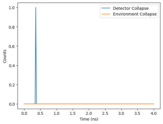
The following code provides a simple example of how to interpret the output. The call to output.col_which[x] returns a list of which collapses occured on the xth trajectory, and to output.col_times[x] returns a list of the time of each those collapses. The value of output.col_which indicates the collapse operator corresponding to the collapse event – in this case a value of 0 represents a detection event, and a value of 1 represents a collapse to the environment.
D1 = np.zeros(time_scale+1) #histogram of detection events in detector 1 -- here associated with the zeroth collapse operator.
E1 = np.zeros(time_scale+1)
i0 = 5 #randomly chosen trajectory index

index = len(output.col_which[i0]) #length of ouput collapse events at chosen trajectory

# -- Loop over output vector at trajectory index i0
# -- If event is found associated with the detector (index 0),
# -- increment the count at that time by 1
for j in np.arange(index):
  if (output.col_which[i0][j] == 0):
    D1[int(output.col_times[i0][j]/tres)] += 1
  if (output.col_which[i0][j] == 1):
    E1[int(output.col_times[i0][j]/tres)] += 1

plt.plot(t,D1,label='Detector Collapse')
plt.plot(t, E1, label='Environment Collapse')
plt.legend(loc='upper right')
plt.ylabel('Counts')
plt.xlabel('Time (ns)')
plt.show();
Questions#
1a. Plot the detector counts over a random set of 10 trajectories based on the output of the Quantum Monte Carlo simulation. Plot time on the x-axis and which collapse occured on the y-axis.
1b. Plot the detector counts over time when summing over all the quantum Monte Carlo trajectories. This should be a histogram of counts over time.
1c. Thinking of trajectories as individual experiments, investigate the mean and variance of the number of photons collected in blocks of 50 measurements at a time. Consider the ratio of the variance divided by the mean number of photons per block.
Coherent laser sources emit photons according to a Poisson process. What is this ratio for a Poisson process? What do you observe? What distribution is your observation consistent with?
1d. Re-run the above simulation with different atom-cavity coupling, \(g_0\), say 0.5, 1, and 2. Plot your results and explain what you observe.
1e. We would next like to investigate the statistics of the photons being emitted by this system. One common way of doing this is by using an auto-correlation measurement where we measure a time delay between the single photon detection events while the atom is continuously excited (i.e. \(g^{(2)}(\tau)\)). We can model the excitation with a semi-classical field of the form
Modify the single emitter code above to include the emitter driving using \(g_0=2\) and \(\Omega=.5\). For each Monte Carlo trajectory, count the the delay between every single photon event pair (incldue zero and negative delays) and show a histogram of the result. Explain why the histogram has the shape it does. How do you think this would change if you had two driven emitters coupled to the cavity mode?
We get you started by setting up the Hamiltonian and solver below, after which you can add the code for the auto-correlation.
# 1e ***solution***
psi0 = tensor( basis(N,0), excited )
numb = 5000

g1 = .5
HD = g1 * ( sigma.dag() + sigma ) # time-independent Hamiltonian of system A

output = mcsolve([H0_A, HD], psi0, t, c_ops, e_ops, ntraj = numb, progress_bar=True)
2. Two-Emitter interference#
We would now like to simulate what happens when we interfere the photons from two emitters, A & B, in a Hong-Ou-Mandel (HOM) experiment shown schematically in the figure below. In this case we drive the emitters with excitation pulses tuned to generate only up to one photon per pulse. With identical excitation and mixing through the beamsplitter in a way such that they are indistinguishable afterwards, you are able to generate a NOON state at the output with \(N=2\). This can be observed by again analyzing correlation events between the two detectors.
Note
In the T3E1 lab you will actually perform a HOM measurment with photon pairs from an SPDC source. For further reference on the HOM measurement and its importance, please refer to the text materials and lecture video on HOM for T3E1

We follow three steps to set up this simulation:
Step 1: Prepare the initial state as the superposition state as: \(|\psi_0\rangle=\frac{1}{\sqrt{2}}\left(|g_{\downarrow}0\rangle_A+|g_{\uparrow}0\rangle_A\right)\otimes\frac{1}{\sqrt{2}}\left(|g_{\downarrow}0\rangle_B+|g_{\uparrow}0\rangle_B\right)\).
Step 2: Excite the emitters with the time-dependent Hamiltonian that uses the semi-classical approximation: $\(\hat{H}_{\text{exc}}\left(t\right)/\hbar=\sum_{s=A,B}P_s(t)(|g_{\downarrow}\rangle\langle e|_s + |e\rangle\langle g_{\downarrow}|_s)\)$
or
where \(P_s\left(t\right)\) is the Rabi frequency of the excitation pulse. For simplicity, let’s assume identical excitation pulses for systems A and B, \(P_A(t) = P_B(t)\).
Step 3: Count the clicks that occur at detector \(D_1\) or \(D_2\), which are placed after a beam-splitter. Note that the beam-splitter mixes the A and B photon modes, such that it measures \((\hat{a}_A+\hat{a}_B)/\sqrt{2}\) and \((\hat{a}_A-\hat{a}_B)/\sqrt{2}\).
In the following, we provide the codes to simulate the photon generation and HOM interferometer.
# Here, let's choose the basis of state as |photon_A, spin_A, photon_B, spin_B>
N = 5 # Set where to truncate Fock state of cavity
sigma_A_gd_e = tensor(qeye(N), ground_down * excited.dag(), qeye(N), qeye(Na)) # |g_down><e| of system A
sigma_B_gd_e = tensor(qeye(N), qeye(Na), qeye(N), ground_down * excited.dag()) # |g_down><e| of system B
sigma_A_gd_gu = tensor(qeye(N), ground_down * ground_up.dag(), qeye(N), qeye(Na)) # |g_down><g_up| of system A
sigma_B_gd_gu = tensor(qeye(N), qeye(Na), qeye(N), ground_down * ground_up.dag()) # |g_down><g_up| of system B
a_A = tensor(destroy(N), qeye(Na), qeye(N), qeye(Na)) # annihiliation operator of system A
a_B = tensor(qeye(N), qeye(Na), destroy(N), qeye(Na)) # annihiliation operator of system B
I = tensor(qeye(N), qeye(Na), qeye(N), qeye(Na)) # Unity operator
We would also like to include some more realistic loss processes, such as cavity loss and non-radiative decay. We can include these through some additional collapse operators,
c_ops = [] # Set of collapse operators
e_ops = []
kappa =0.1 # Cavity decay rate
c_ops.append(np.sqrt(kappa) * a_A) # Cavity decay of system A. C0
c_ops.append(np.sqrt(kappa) * a_B) # Cavity decay of system B. C1

gamma =1 # Atomic decay rate
c_ops.append(np.sqrt(gamma) * sigma_A_gd_e) # spontaneous decay (decaying to modes other than cavity) from |e> to |g_down> of system A.   C2
c_ops.append(np.sqrt(gamma) * sigma_B_gd_e) # spontaneous decay (decaying to modes other than cavity) from |e> to |g_down> of system B.   C3

K_c = 10 # rate for collapsing to detector
c_ops.append(np.sqrt(K_c) * (a_A+a_B)/np.sqrt(2)) # Collapsing to detector 1        C4
c_ops.append(np.sqrt(K_c) * (a_A-a_B)/np.sqrt(2)) # Collapsing to detector 2        C5
numb=200 # numbers of trajectories (affects runtime)
time_scale=200
tmax = 4.0 # (ns)
t = np.linspace(0.0, tmax, time_scale+1) # Define time vector (0 to 4ns, 20ps resolution)

# Step 1
theta=np.pi/4
photon = basis(N, 0) # Initial photonic state
spin = ground_down*np.cos(theta)+ground_up*np.sin(theta) # Initial spin state
psi0 = tensor(photon, spin, photon, spin) # Initial global state

g0 = 2 # coupling strength (Rabi frequency of vacuum field)
# Here describes the interaction Hamiltonian
H0_A = -g0 * (sigma_A_gd_e.dag()*a_A + a_A.dag()*sigma_A_gd_e) # time-independent Hamiltonian of system A
H0_B = -g0 * (sigma_B_gd_e.dag()*a_B + a_B.dag()*sigma_B_gd_e) # time-independent Hamiltonian of system B
H0 = H0_A + H0_B # time-independent Hermitian of global system

# Here describes the excitation Hamiltonian
H1_A = (sigma_A_gd_e.dag() + sigma_A_gd_e) # time-dependent Hamiltonian of system A after semi-classical approximation
H1_B = (sigma_B_gd_e.dag() + sigma_B_gd_e) # time-dependent Hamiltonian of system B after semi-classical approximation
e_ops.append(ket2dm(psi0).dag()* (ket2dm(psi0)))

# Excitation pulse parameters
center=0.6
life_time=0.2
peak =np.sqrt(np.pi)/2/life_time
excite_pulse_A = peak * np.exp(-((t-center) / life_time) ** 2)
excite_pulse_B = peak * np.exp(-((t-center) / life_time) ** 2)
#print(excite_pulse_A)
#Step 2
H = [H0,[H1_A, excite_pulse_A],[H1_B, excite_pulse_B]]
output = mcsolve(H, psi0, t, c_ops, [], ntraj = numb, progress_bar=True)
Questions#
2a: Adapt the code from before to get the counts in detectors 1 & 2 over time (summing across all trajectories).
Let’s take a look at the experimental HOM interefernce data from Zhai, Liang, et al. “Quantum interference of identical photons from remote GaAs quantum dots.” Nature Nanotechnology 17.8 (2022): 829-833.

Here, Zhai et al. are repeatedely applying excitation pulses to two emitters A/B, and measuring the difference in time (\(\tau\)) between counts in detector D1/D2. This is called a correlation, or \(g^2(\tau)\) measurement. Your code simulates only a single pulse, corresponding to the centermost pulse in this result. Let’s explore the statistics observed in this plot for ourselves below.
2b: Suppose you have an initial cavity mode state \(\hat{a}^\dagger_A\hat{a}^\dagger_B|0\rangle\) (one photon in each A,B). By the beamsplitter transformation, the output modes have operators given by \(\hat{c} = (\hat{a}+\hat{b})/\sqrt{2}\) and \(\hat{d} = (\hat{a}-\hat{b})/\sqrt{2}\). What is the final state of the photon modes in terms of the output modes? If you were to detect these photons, what properties would they have? How does this relate to the HOM correlation at \(\tau=0\)?
Hint: write \(\hat{a}\) and \(\hat{b}\) in terms of \(\hat{c}\) and \(\hat{d}\).
2c. Write the code for calculating the second order coincicent counting \(g^2\)(\(\tau\)) for the central peak. Plot the result.
Hint: Look at coincidences (where one photon goes to each detector) within each trajectory.
2d. Write the code for calculating the second order coincicent counting \(g^2\)(\(\tau\)) for the side peak. Plot the result.
Hint: Wait, we said you are only simulating a single pulse? That’s true, but you have many trajectories which are effectively different experiments, so you can assume that neighbouring Monte Carlo trajectories come from different excitation pulses!
2e: In the case where the photons have perpendicular polarisations, what should \(g^2_{\perp}(0)\) be?
To quantify the quality of the photon interference, we can define the visibility:
\(g^2_{||}\) = \(I_{\text{central peak}}/I_{\text{side peak}}\) (For || case)
\(g^2_{\perp}\) = \(I_{\text{central peak}}/I_{\text{side peak}}\) (For \(\perp\) case, which the result of 2e can be used)
\(V=1-g^2_{||}/g^2_{\perp}\)
2f: Calculate the visibility based on your result in 2b and 2c. Why do you think the visiblity isn’t 1?