TEXT – Interference, Entanglement and Quantum-Enhanced Metrology

In this chapter we examine entangled photon pair generation, single-photon interference, entangled photon pair interference by way of the Hong-Ou-Mandel effect, and entangled multi-photon Fock state interference for quantum-enhanced phase sensing. Along the way we will discuss basic principles important to a variety of areas in quantum photonics, such as: the interaction of photons with beamsplitters; the interference of photon number states; signal detection and processing methods such as coincidence detection; and how to analyze statistical fluctuations of photon detection events for determining sensitivity and signal to noise ratio in measurements.

The information and techniques discussed here will not only be useful for your lab exercises, but will be critical tools that you can leverage for your final projets.

Pre- and Post-Labs

This lab has three pre-labs and one post-lab. The pre-labs are due at the start of lab sessions 1-3. The post-lab can be turned in with your final summary report.

Entangled Photon Pair Generation and Measurement

You will work with entangled photon pairs that are generated using SPDC. This process is also described in the T2E1 material in more technical detail, and you can also read the information in the QuED manual which is quite helpful. Here we will stick to the most important aspects important to understanding the emitted photons and how we can use them.

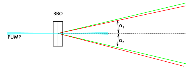
Fig. 5 Simplified schematic of the SPDC source that you will use in the lab and possible cone angles of the entangled photon pair outputs from the crystal.

An SPDC source similar to what you will use is shown in Fig. 5. Note that when excited by the pump that is at a higher energy of \(2\hbar\omega\), two photons of energy \(\hbar\omega\) are generated in a cone of angles away from the crystal. In our systems, as shown here, two crystals are stacked together, one generating entangled photons with horizontal polarization, and one with vertical polarization. This generation process is quantum-coherent, and the state that arises is in a superposition of these photon pairs, and we can write it as

\[ \ket{\psi} = \frac{1}{\sqrt{2}} \big\lbrace \ket{H}_a\ket{H}_b + \ket{V}_a\ket{V}_b\big\rbrace\]

Where we have taken the top path to be path \(a\) and the bottom to be path \(b\). To get a feeling for the entanglement, consider a simple experiment as shown in Fig. 6.

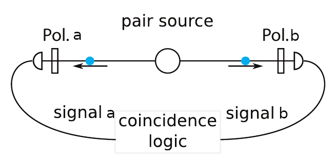
Fig. 6 Schematic of an entanglement experiment.

Each path is sent through a polarizer and then a detector after which we consider only coincident events. Let’s now consider the act of measuring the photons after the polarizers in arms \(a\) and \(b\). The polarizer acts to select out only one polarization angle. Since our incident light has both polarizations, we need to understand how both components are projected onto the polarization axis.

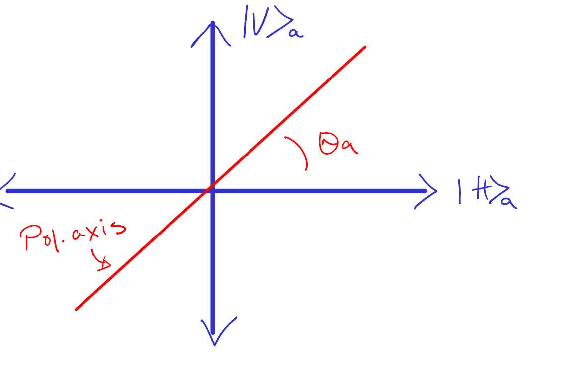
Fig. 7 The horizontal and vertical polarization states are projected onto the polarizer axis denoted by the red line.

Consider Fig. 7. This shows the polarizer angle in arm \(a\) in relation to the vertical and horizontal polarizations of our input photons. After the polarizer, the light must be polarized along \(\theta_a\), and we can write:

\[\ket{\theta_a} = \cos(\theta_a)\ket{H}_a + \sin(\theta_a)\ket{V}_a\]

The same expression also applies to \(\ket{\theta_b}\). In our measurement, we are considering coincident events that correspond to states \(\ket{\theta_a}\ket{\theta_b}\). To find the probability of detecting such states, we simply project this state onto our input state and take the square magnitude. The probability of coincidences \(P_\text{co}\) is then

\[P_\text{co} = \frac{1}{2} \Big | \bra{\theta_a}\bra{\theta_b} \big\lbrace \ket{H}_a \ket{H}_b + \ket{V}_a \ket{V}_b\big\rbrace \big |^2\]

We leave it as an exercise to show that \(P_\text{co} = \frac{1}{2} \cos^2(\theta_a - \theta_b)\).

Think about what this is saying for a bit. No matter how far apart your detectors are, by setting the polarization in one arm, you instantly dictate the joint probability which also requires an event at the detector in the other arm and depends on its polarization axis. While correlations can also exist in classical systems, this specific correlation pattern cannot be explained classically. It violates Bell’s inequality indicating that the input state exhibits quantum entanglement.

In the lab, we will perform this experiment so that you can experience entanglement for yourself.

Prelab 1 Questions

1. Fill in the missing steps above to show that \(P_\text{co} = \frac{1}{2} \cos^2(\theta_a - \theta_b)\).

2. Make a polar plot of \(P_\text{co}\) as a function of \(\theta_a\) for three fixed settings of \(\theta_b\). Interpret what the plots are saying.

3. In the lab, our SPDC process generates on the order of 100,000 photon pairs per second. Is there any chance in our measurements that a neighboring photon might influence our results? Justify your answer.

4. Describe, from an engineering perspective, why entanglement is important. Provide examples.

Single-Photon Interference

In the following text we discuss single photon interference. We start with an examination of photon number transmission through an interferometer. We discuss this result in the context of an interaction-free measurement. We then discuss measurement noise in the photon number detection at the interferometer with a partial absorber, and the role of the vacuum state inputs and their impact on this noise. Finally we discuss the concept of photon frequency bandwidth and the impact that has on the nature of the interference.

Beyond the lecture videos provided below, an excellent lecture on single-photon interference can also be found here.

Single-Photon Transmission Through an Interferometer and Interaction-Free Measurements

Before moving on to multiple-particle interference, let us now consider single-particle interference. We will also discuss how in this single-particle case one can achieve measurement without interaction.

Consider the single-photon interferometer as shown in Fig. 8

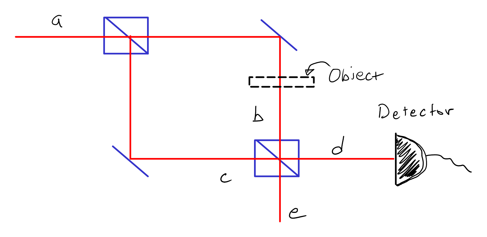
Fig. 8 Interferference of a single photon in a Mach-Zender interferometer. An optional absorbing object can be placed in one of the paths.

For dealing with interference here and below, we will track the annihilation operators through the system. For a refresher on how these work, see the BASICS chapter on quantum optics.

Our strategy is to develop a description of the annihilation operator of the output state using the annhihilation operators of the input states of the first beamsplitter. This description can then be used to determine the number of output photons going to the detector based on the input states. Note that for this problem we consider that only one input of the beasmplitter is excited by a single photon (denoted as \(a\)). While a rigorous solution would have to account for all annihilation operators, including that of the vacuum state input to the first beamsplitter, the operators of the vacuum state inputs do not contribute to the average photon number at the detector (however they can contrubute to noise in the photon detection as we discuss in the following sections). Since we are concerned with the photon number for the purposes of this discussion, we drop the operators associated with the vacuum input as a shorthand which simplifies the analysis. It is emphasized that you would need to include all input operators to describe the input and output states completely, or to calculate detection noise properties for a general set of input states. See the note below for further reading.

Note

For an interseting discussion of how the vacuum state input contributes to photon fluctuations, and how these fluctuations can be reduced using squeezed light, see the discussion of homodyne detection with squeezed light in EXTRAS – Homodyne Detection

Taking each path \(b\) and \(c\) individually, we find that for path \(b\) the annihilation operator going into the second beamsplitter, ignoring the annihilation operator of the empty port, can be written as

\[\bhat = \alpha e^{i\phi_b} \ahat/\sqrt{2}\]

Likewise

\[\chat = e^{i\phi_c} \ahat/\sqrt{2}\mathrm{.}\]

The phase is the phase accumulated during propagation in each path and scales as \(2\pi l /\lambda\), where l is the path length in either arm. The term \(\alpha\) accounts for loss in interaction with the object. This could in general be a complex amplitude, but here we simply assume it is real noting the amount of absorption in the object (the phase can be wrapped into the total phase in the path).

We now want to know waht the annihilation operator for \(d\) is going to our detector. The beamsplitter has the relation that

\[\dhat = \frac{1}{\sqrt{2}} ( \bhat + \chat )\]

and likewise

\[\ehat = \frac{1}{\sqrt{2}} ( \bhat - \chat )\]

Let’s focus on path \(d\) and find the number of photons going there. The photon number operator is given by \(\ddagger \dhat\). We can now express this as

\[\ddagger\dhat = \frac{1}{4} ( \adagger\ahat + \alpha e^{-i\Delta\phi} \adagger \ahat + \alpha e^{i\Delta\phi} \adagger\ahat + \alpha^2 \adagger\ahat )\]

where we have that \(\Delta\phi\) is the phase difference betwen the paths \(b\) and \(c\). We leave this as an exercise to show.

Reducing this we find that

\[\ddagger\dhat = \frac{1}{4} \bigg ( 1 + \alpha^2 + 2 \alpha \cos(\Delta\phi) \bigg ) \adagger\ahat\]

So now, we finish by finding the photon number expectation at the output \(N_d\) for a single photon in \(a\) at the input.

\[N_d = \bra{1}_a \frac{1}{4} \bigg ( 1 + \alpha^2 + 2 \alpha \cos(\Delta\phi) \bigg ) \adagger\ahat \ket{1}_a\]

which reduces to

\[N_d = \frac{1}{4} \bigg ( 1 + \alpha^2 + 2 \alpha \cos(\Delta\phi) \bigg )\mathrm{.}\]

Let’s consider two important cases: \(\alpha = 1\) (no object), and \(\alpha = 0\) (opaque object). For \(\alpha = 1\) we have that the probability oscillates sinusoidally with the phase difference \(\Delta\phi\). We can control this with a wedge or the movement of one of the mirrors in the lab.

Note

Here we have considered states containing only a single frequency, meaning that interference would continue indefinitely with increasing delay. However, in reality our states contain a distrubtion of frequencies and exhibit finite coherence times that limit the range of delays over which one could observe this interference. In experiment we will find that the interference fringes disappear after several wavelengths of delay. For our case this is due to the relatively large bandwidth of frquencies generated in the SPDC process.

The case of a non-zero bandwidth is also treated in .

It also makes sense that when \(\alpha = 0\) all interference goes away, and we are left with only 1/4 of the photons making it to the detector. The other 1/4 go to arm \(e\), and the other half are lost to the object.

Now for something interesting. Let’s say that we align our interferometer without an object in place such that you have a minum probability of finding the photons in arm \(d\). That would be for \(\Delta\phi = \pi\) so that no photons are output. Then you put the object in place – the photon expectation suddenly goes to 1/4. You just detected the object without interaction! This is in fact often referred to as an interaction-free measurement, and has found renewed interest in the context of electron detection where particle energies are high and damage per particle can be significant.

In the questions below, you will consider such measurements further.

Rigorous Solution of Mach-Zender Interferometer

In the previous discussion, we took a shortcut to calculating the photon number expectation by ignoring the operators of the vacuum state inputs. This simplifies the problem, but is not a rigorous solution. A particular shortcoming is that this approach would give incorrect results for calculating the noise properties of the photon number at the detectors as in that case the vacuum state input does matter. Here we discuss the rigorous solution. We start without an absorbing object, and then inroduce how we can accurately model an absorbing object to accurately account for the quantum noise introduced by it.

Complete solution without an object

The problem setup is the same as before, however now we must include all inputs, which slightly modifies our setup as shown in Fig. 9.

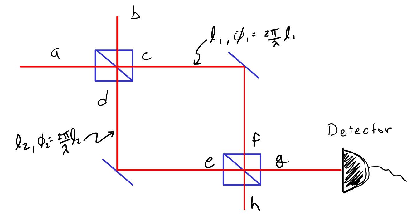
Fig. 9 Considering all inputs and outputs for the complete description of the Mach-Zender interferometer.

Now we can proceed to find the annihilation operators as before, but with all inputs included.

\[\chat = \frac{\ahat + \bhat}{\sqrt{2}}\]

and

\[\dhat = \frac{\ahat - \bhat}{\sqrt{2}}\mathrm{.}\]

We then account for propagation over paths \(l_1\) and \(l_2\) which lead to a phase shift of \(\phi_n = 2 \pi l_n/\lambda\).

\[\ehat = \dhat e^{i\phi_2}\]

and

\[\fhat = \chat e^{i\phi_1}\mathrm{.}\]

From here, we account for the fact that at the second beamsplitter we have

\[\ghat = \frac{\ehat + \fhat}{\sqrt{2}}\]

and

\[\hhat = \frac{\ehat - \fhat}{\sqrt{2}}\mathrm{.}\]

After substituting everything in we get the final expression for \(\ghat\):

\[\ghat = e^{i\phi_2} e^{i\Delta\phi/2} \bigg \lbrace \ahat \cos(\Delta\phi/2) + i \bhat \sin(\Delta\phi/2) \bigg \rbrace \]

where \(\Delta \phi = \phi_1 - \phi_2\), the phase difference between the two arms.

Note that the number operator for \(g\) is then:

\[\gdagger \ghat = \cos^2(\Delta \phi /2)\adagger\ahat + j\adagger\bhat \cos(\Delta\phi/2)\sin(\Delta\phi/2) - j\bdagger\ahat \cos(\Delta\phi/2)\sin(\Delta\phi/2) + \bdagger\bhat \sin^2(\Delta\phi/2) \mathrm{.}\]

Given our input state is \(\ket{1}_a \ket{0}_b\), the photon number is then found by taking:

\[N_g = \bra{0}_b \bra{1}_a \gdagger \ghat \ket{1}_a \ket{0}_b = \frac{1}{2} \lbrace 1 + \cos(\Delta\phi ) \rbrace \mathrm{.}\]

Note that only the terms with \(\adagger \ahat\) have a non-zero contribution – this justifies our neglecting the vacuum-state inputs for calculation of the output photon number.

However, it we emphasize that you must use this more complete treatment and account for the vacuum-state inputs to accurately predict the quantum noise in systems. For example, the standard deviation of the photon number depends on \(\hat{N}^2\) (see the note in Mean and Standard Deviation Observables), and the vacuum state inputs can contribute to the expectation \(\left < \hat{N}^2 \right >\). As a further example, to see the importance of the vacuum state input in interferometry, please see the use of squeezed vacuum to reduce quantum noise as described in EXTRAS – Homodyne Detection.

Accounting for the partial absorber

For the partial absorber, again our treatment in the text was adequate for accounting for the outgoing photon number. However, a rigorous solution requires accounting for the vacuum state here again.

The partial absorber can in fact be modeled as a beamsplitter with adjustable transmission/reflection with one input being the vacuum state, the other being the input state, and one output going to a perfect absorber, and the other transmitting out. See Fig. 10.

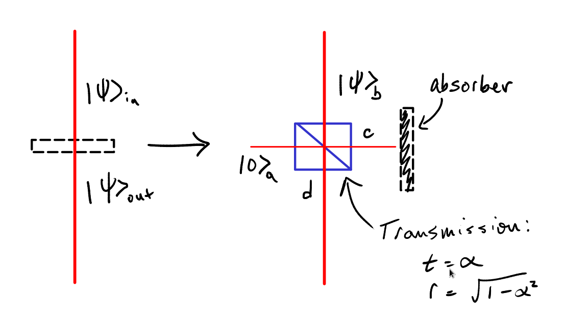
Fig. 10 Model of a partial absorber using a beamsplitter to account for the vacuum state.

This model accounts for the vacuum state properly. Note here the beamsplitter is not a 50:50 beamsplitter to account for the adjustable transmission probability. The input/output relations are similar, with:

\[\chat = t\ahat + r\bhat\]

and

\[\dhat = r\ahat - t\bhat \mathrm{.}\]

From the derivation in the text, we have that \(t = \alpha\), and \(r = \sqrt{1 - \alpha^2}\). You can show that with this element in the Mach-Zender interferometer, the output photon number expectation is equivalent to what we derived, with the number of detected photons being

\[N_d = \frac{1}{4}\lbrace 1 + t^2 + 2t\cos(\Delta \phi)\rbrace \mathrm{.}\]

However, as noted earlier, the impact of this absorbing object is to effectively couple in vacuum state which must be accounted for during analysis of the quantum noise limit of the interferometer.

Accounting for Bandwidth

Finally, let us address the issue of the state having a non-zero bandwidth. Up until now, we have discussed states from the context of a single frequency. Our results would imply that interference would continue indefinitely as one changes delay. However, in practice our source states will have a non-zero bandwidth which leads to a finite range of delays over which one would observe interference. In this section, we will introduce how to account for this bandwidth.

For the case of a non-zero bandwidth, we can write our single-photon input state as

\[ \ket{\psi_\mathrm{in}} = \int_{-\infty}^\infty \mathrm{d}\omega \phi(\omega) \ket{1;\omega}_a \mathrm{,}\]

where \(\phi(\omega)\) contains the spectral amplitude and phase distirubtion for each frequency component. Note that by normalization we have that

\[\braket{\psi_\mathrm{in}}{\psi_\mathrm{in}} = \int_{-\infty}^\infty \mathrm{d}\omega_1 \int_{-\infty}^\infty \mathrm{d}\omega_2 \phi(\omega_2)^{*} \phi(\omega_1) \braket{1;\omega_2}{1;\omega_1}_a \]

Given orthonormality we have that \(\braket{1;\omega_2}{1;\omega_1}_a = \delta(\omega_2 - \omega_1)\), which removes the second integral, simplifying everything to

\[\braket{\psi_\mathrm{in}}{\psi_\mathrm{in}} = \int_{-\infty}^\infty \mathrm{d}\omega_1 |\phi(\omega_1)|^2 = 1\]

What is this all saying? Basically, we are saying that we have a probability of 1 of finding a photon over a range of frequncies defined by the distribution \(|\phi(\omega)|^2\). While we will always find a photon, we just don’t know for certain what energy it has due to the finite bandwidth of our source.

Taking this further, we can define the state in terms of the creation operator.

\[ \ket{\psi_\mathrm{in}} = \int_{-\infty}^\infty \mathrm{d}\omega \phi(\omega) \adagger(\omega) \ket{0}_a \mathrm{.}\]

In this way, we can track the operators through any system in the same way as we already have for the single-frequency states. Following this method, we can re-express our output state calculated from our earlier analysis of the interferometer now accounting for the non-zero bandwidth:

\[\ket{\psi_\mathrm{out}} = \int_{-\infty}^\infty \mathrm{d}\omega \cos \bigg ( \frac{\omega \Delta l}{2c} \bigg )\phi(\omega) \ket{1;\omega}_a \mathrm{.}\]

Note that here it is important as we write the phase difference in terms of \(\omega\) and the path length difference \(\Delta l\). What is the probability of finding a photon then. Well, we just take \(\braket{\psi_\mathrm{out}}{\psi_\mathrm{out}}\), which becomes

\[\braket{\psi_\mathrm{out}}{\psi_\mathrm{out}} = \int_{-\infty}^\infty \mathrm{d}\omega_1 \int_{-\infty}^\infty \mathrm{d}\omega_2 \phi(\omega_2)^{*} \phi(\omega_1) \cos \bigg ( \frac{\omega_1 \Delta l}{2c} \bigg )\cos \bigg ( \frac{\omega_2 \Delta l}{2c} \bigg )\braket{1;\omega_2}{1;\omega_1}_a \]

Again, we have that \(\braket{1;\omega_2}{1;\omega_1}_a = \delta(\omega_2 - \omega_1)\), and after substitution this again gets us back to one integral:

\[\braket{\psi_\mathrm{out}}{\psi_\mathrm{out}} = \int_{-\infty}^\infty \mathrm{d}\omega_1 |\phi(\omega_1)|^2 \cos \bigg ( \frac{\omega_1 \Delta l}{2c} \bigg )^2 \mathrm{.}\]

Note that the major difference here is the adddition of the cosine term. This resuts in an oscillation of the output photon detction probability. Note that the bandwidth probability distirubution function \(\phi\) then dictates the range of delays over which you see this oscillation in probability. Importantly, note that that all phase information inside of \(\phi\) is lost as the output is dictated by \(|\phi|^2\) (our interferometer is, after all, only sensitive the phase differences between the two arms, and not to the absolute phase of the incoming state).

Let’s now numerically explore the single-photon interference accounting for bandwidth.

We start by taking a Gaussian distribution for \(\phi\).

import numpy as np
import matplotlib.pyplot as plt

# -- Settings -- 
c  = 300 #speed of light in nm/fs
lambda_0 = 810 # central wavelength in nm
sigma = 0.3 # bandwidth of the photons in petahertz
omega_0 = 2*np.pi*c/lambda_0 #central frequency of the photons

# -- Calculations

#Set up the frequency axis (rad/fs)
omega = np.linspace(omega_0 - 10*sigma, omega_0 + 10*sigma, 10000)

#Define the initial gaussian frequency distribution
phi = np.exp(-(omega - omega_0)**2/sigma**2)

#Ensure it is normalized properly
norm_factor = np.sqrt(np.trapz(np.abs(phi)**2, x = omega))
phi = phi/norm_factor

#Plot for visualization
fig = plt.figure()
plt.plot(omega, abs(phi)**2, label=r'$\phi(\omega)$')
plt.legend(fontsize=13)
plt.xlabel(r'$\omega$ (rad/fs)', fontsize=13)
plt.ylabel(r'$\phi(\omega)$', fontsize=13);

fig.set_size_inches(10, 7)

Show code cell output Hide code cell output

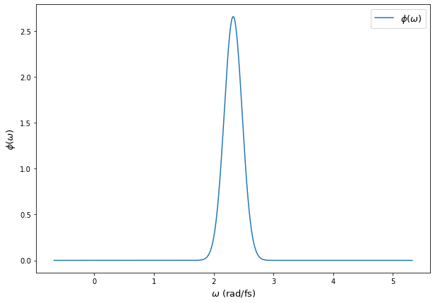
Fig. 11 Normalized spectral distribution of single-photons.

Next, we define the path length difference and perform the integral for each choice of delay.

#-- Settings -- 

#Define the delay length (in nm)
l = np.linspace(-10e3, 10e3, 1000) #Path length difference to scan over

# -- Calculations -- 

#Set up vector for output probabilities
P_out = np.zeros(l.shape) #Probability of seeing a photon at the output

#Now calculate output probability for each delay
for cc in range(0, l.size):

    P_out[cc] = np.trapz(np.abs(phi)**2*np.cos(omega*l[cc]/2/c)**2, x = omega)

fig = plt.figure()
plt.plot(l, P_out)
plt.xlabel('delay length (nm)', fontsize=13)
plt.ylabel('photon detection probability', fontsize=13);

fig.set_size_inches(10, 7)

Show code cell output Hide code cell output

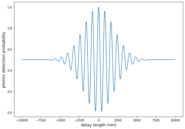
Fig. 12 Single-photon interference as a funciton of delay with finite bandwidth.

Prelab 2 Questions

1. Fill in the missing steps to get to the expression for \(\ddagger\dhat\) above.

2. Write the corresponding expression for the number of expected photons exiting path \(e\).

3. Discuss the interaction-free measurement in the context of a translucent object (\(0 < \alpha < 1\)).

4. Read about the Elitzur-Vaidman bomb test. Explain how, when performed photon by photon and with a detector at ports \(d\) and \(e\) a probability of detection without interaction can approach 33 percent. Justify your answer.

5. Using the rigorous solution of the operator describing the output port to the detector, calculate the variance in the output for \(\alpha = 0\), \(\Delta N = \left < \hat{N}^2 \right > - \left < \hat{N} \right >^2\). Note that at the output you have either a detection event or not – this is like a coint toss which follows a binomial distribution with variance \(P(1-P)\), where \(P\) is the probability of detection. Does your variance calculated using the operators make sense based on this?

Interference of Two Single Photons: The Hong-Ou-Mandel Effect

We have now examined how a single photon interferes with itself, but how do two single coincident photons interfere with each other at a beamsplitter? In this section we explore such two-photon interference. We examine how when the two photons are indistinguishable in every way, the interference can lead to photon bunching and anti-correlation at the output ports. The outgoing state generated is referred to as a two-photon NOON state of the form \(\frac{1}{\sqrt{2}} ( \ket{N}_a\ket{0}_b + \ket{0}_a\ket{N}_b )\). Pushing beyond this observation, in the text that follows this section we examine how NOON states can generally be used for quantum-enhanced sensing.

Imagine the scenario depicted in Fig. 13. A nonlinear crystal is used to generate precisely two photons of energy \(\hbar\omega\) when excited by a pulse with a photon energy of \(2\hbar\omega\). This process is called spontaneous parametric down-conversion and is a common technique for generating entangled photon pairs.

The two photons travel away from the crystal along two paths (top and bottom as shown). They are then brought together and interfere within a beamsplitter.

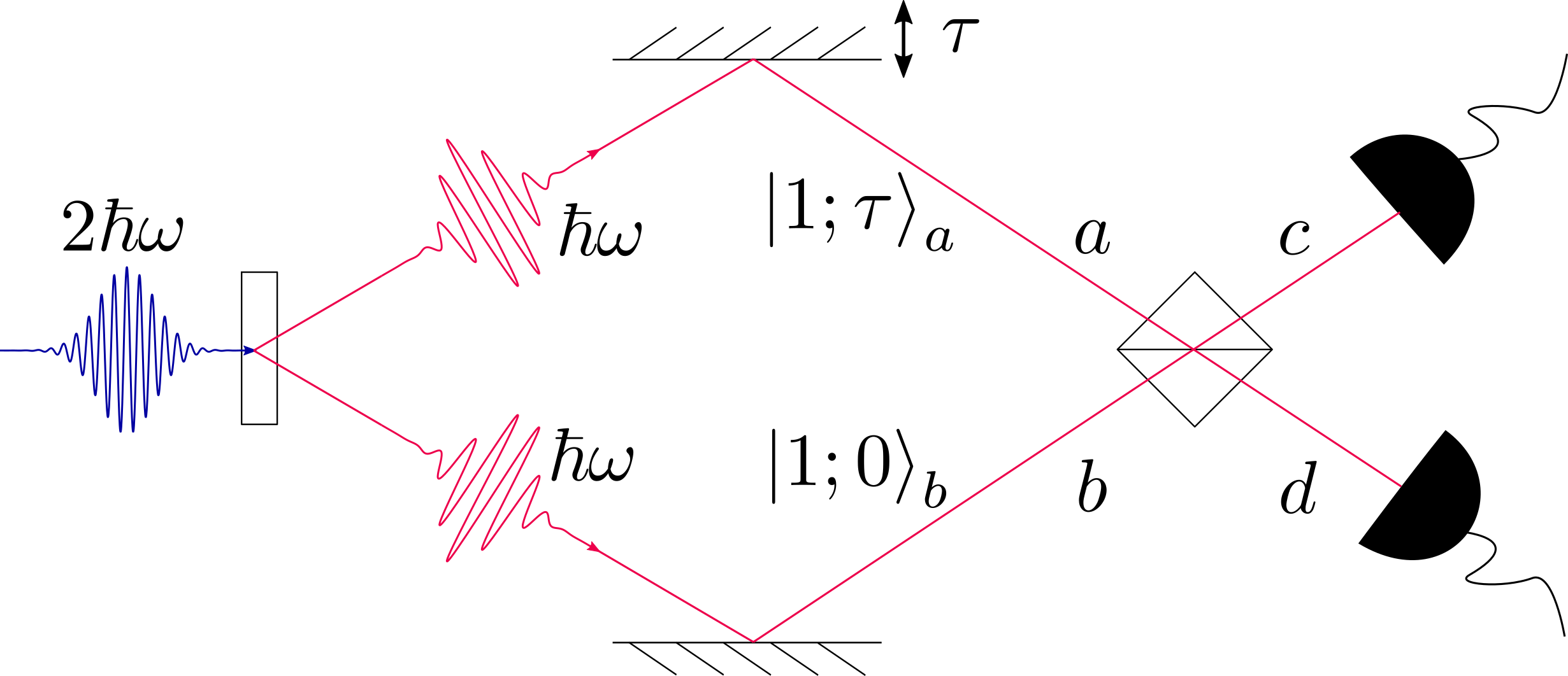
Fig. 13 Experimental setup for studying the HOM effect.

If we break down all the different possibilities that could happen, one would be that both photons output in \(c\), another would be that both photons output in \(d\), and a final possibility would be that one photon outputs to \(c\) while the other outputs to \(d\). One interesting question to ask is whether the delay has any influence over these possibilities?

Lets model this system. Imagine that the input signals are pulsed. In this case we could for instance represent a single photon input with delay \(\tau\) in port \(a\) as

\[ \ket{1; \tau}_a, \]

or a single photon input with \(0\) delay in port \(b\) as

\[ \ket{1; 0}_b.\]

The first number represents the numer of photons, the second the delay. Finally, the subscript represents the mode. Given an entangled two-photon input to the system from the crystal with delay along path \(a\) of \(\tau\), we have that the input state can be written as

\[\ket{\psi_\text{in}} = \ket{1; \tau}_a\ket{1; 0}_b = \adagger_{\tau}\bdagger_0 \ket{0}\]

It is important here that the state be written as a tensor product as it captures that the two photons are jointly created and entangled which is the case for the photons generated with SPDC.

Note

We have taken a little liberty here to assign creation and annihilation operators for each mode with their mode label. It’s just a bit of shorthand that is very common to make things easier to read if there are only a handful of modes to deal with.

Now we need to understand how such an entangled state interacts with a beamsplitter. For this we will keep track of the different creation/annihilation operators through the system.

A beamsplitter has the following relationship between the input and output modes:

\[\ahat_\tau \rightarrow \frac{\chat_\tau + \dhat_\tau}{\sqrt{2}},\]

and

\[\bhat_0 \rightarrow \frac{\chat_0 - \dhat_0}{\sqrt{2}},\]

thus, the output state becomes

\[ \ket{\psi_\text{out}} = \frac{1}{2} \bigg \lbrace \cdagger_\tau \cdagger_0 - \cdagger_\tau \ddagger_0 + \ddagger_\tau \cdagger_0 - \ddagger_\tau \ddagger_0 \bigg \rbrace \ket{0} \]

Let’s start for the case of \(\tau \neq 0\). In this case we have that

\[ \ket{\psi_\text{out}} = \frac{1}{2} \bigg\lbrace \ket{1;\tau}_c\ket{1;0}_c - \ket{1;\tau}_c\ket{1;0}_d + \ket{1;0}_c\ket{1;\tau}_d - \ket{1;\tau}_d\ket{1;0})_d \bigg\rbrace. \]

Remember that probabilities of outcomes are related to \(\braket{\psi_\mathrm{out}}{\psi_\mathrm{out}}\), thus we can make the following map of outcomes at each detector.

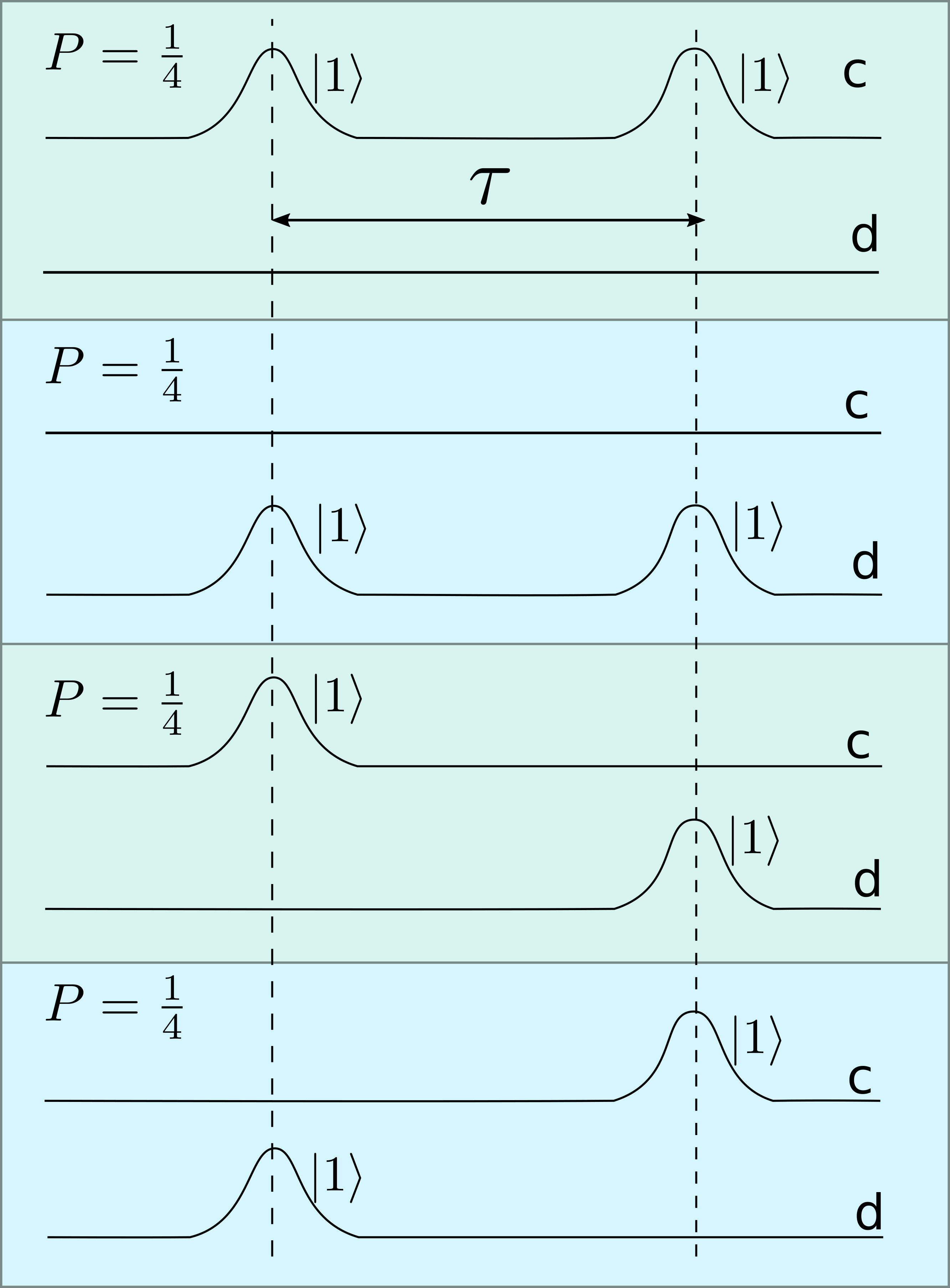
Fig. 14 Four different possibilities of detection in port c and d given a non-zero delay \(\tau\).

All possibilities we oultined above happen with equal probability.

However, for \(\tau = 0\) we have something very interesting, and a bit unintuitive. In this case we have

\[ \ket{\psi_\text{out}} = \frac{\sqrt{2}}{2} \bigg\lbrace \ket{2;0}_c - \ket{2;0}_d \bigg\rbrace \]

leading to the following map of outcomes at each detector.

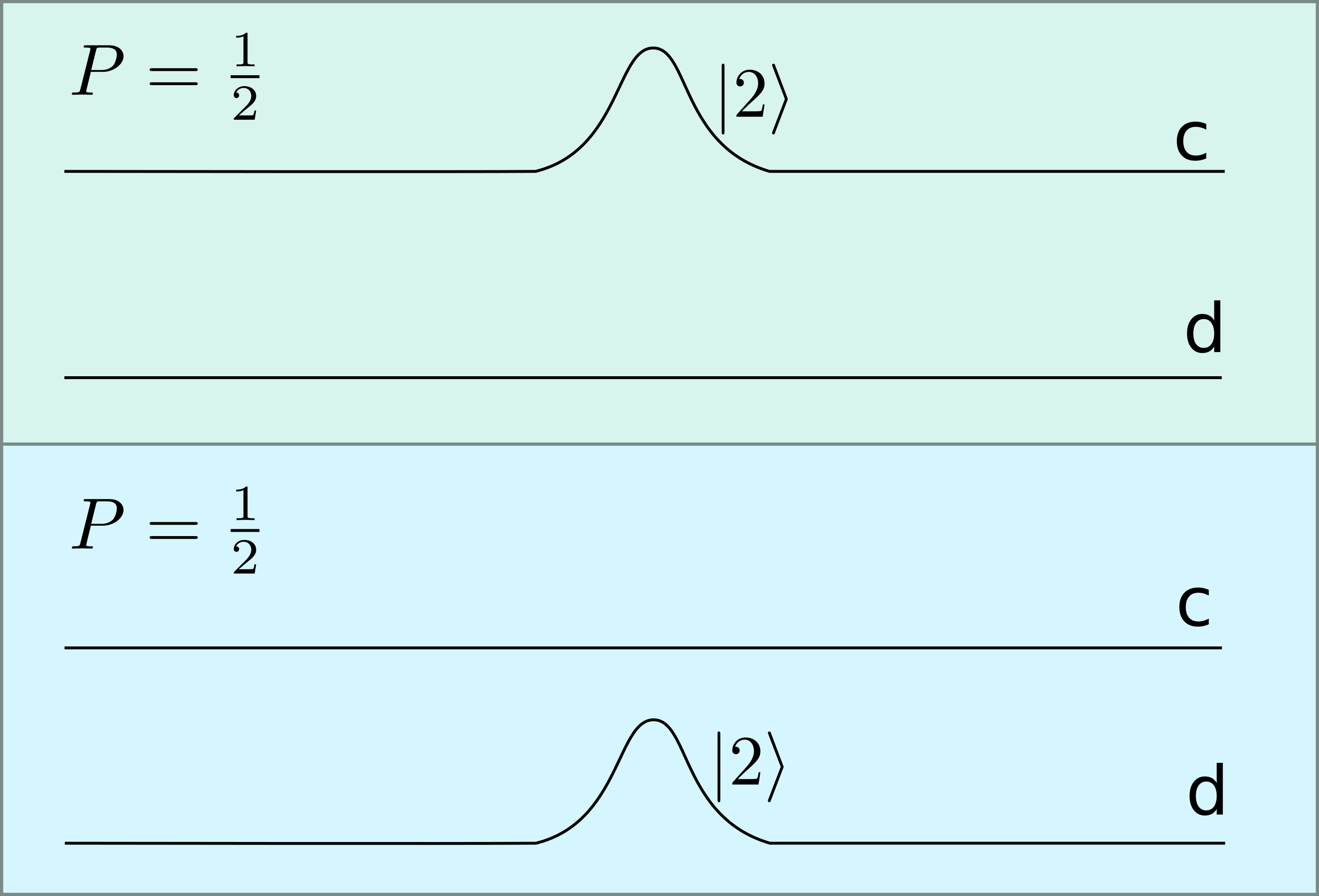
Fig. 15 Two different possibilities of detection in port c and d given a zero delay \(\tau\) such that the two photons are indistinguishable in every way at the beamsplitter. Note each pulse now contains two photons, and the probability of each occurance is \(1/2\).

In this case there would be no coincidence events (that is, events that would trigger an output on both detectors). Either both photons go to \(c\) or both to \(d\) with equal probability. This is in contrast to the case when the modes were fully separate in time when the coincidence rate is 50%.

Such two-photon interference was first observed by Hong, Ou, and Mandel in 1987 [HOM87]. In their work, they note that such a measurement allows for the measurement of time intervals between photons with sub-picosecond precision. In the lab, we will also achieve this precision in detecting time-intervals between arriving photon pairs in the observation of HOM interference.

Important

We want to emphasize here that we have taken a few liberties with the notation above. The approach used here works in estimating probabilities for the two cases discussed, assuming (1) that each photon pulse is long relative to the central frequency; (2) that the envelope shape and central frequency of each pulse is the same; and (3) that for the delayed case the photons are so far separated in time that there is no overlap between each photon pulse at the input of the beamsplitter. For these cases the states are either perfectly indistinguishible or distinguishable. A more complete model would actually have to expand each input into the frequency domain and model the interference between each spectral component individually. However this approach is much more involved (e.g. see the treatment in Ref. [Bra17]. In the end, both approaches result in the same predictions as discussed above.

Prelab 3 Questions

1. What happens to the coincidence count rate when the delay is not perfectly zero such that the photon wavepackets are only partially overlapped in time? (Look for experimental measurements of HOM and explain the data over this intermediate delay range in terms of the distinguishability of the states).

2. If the delay is fixed to \(\tau = 0\), but the input photon states have variable polarization \(\ket{\theta_a}\ket{\theta_b}\) what are the output states as a function of the two polarization angles \(\theta_a\) and \(\theta_b\)?

3. Would you expect the coincidence dip to go all the way to 0 in experiment? Why or why not?

Taking Things Further: Quantum Enhanced Sensing with NOON States

Notice that when \(\tau = 0\) the state takes on an interesting superposition of \(N=2\) Fock states. Such states are called NOON states, so here we would have an \(N=2\) NOON state. It turns out that if we send such states through a subsequent interferometer, we can obtain a quantum advantage in sensitivity to phase shifts. In this section, we will explore why this is important and how it works. In the practice problems and exercises, we will also explore limitations to the generalized implementation of this approach and touch on other approaches that are used for similar purposes.

Before we talk about sensing phase shifts, you might be wondering why someone would want to measure optical phase in the first place? Typically, it is not the phase shift itself that we are after, but rather the physical change that has caused the phase shift. A famous example of this is the measurement of gravitational waves using LIGO. In LIGO, extremely small changes in the path length between two arms of an interferometer are caused by a passing gravitational wave. This change in path length manifests as a shift in phase of the light that travels down one arm relative to light that travels down the other. It is just this phase shift that is detected and related to a change in distance. Similar techniques are used on much smaller scales to stabilize fine movements in stages with nanometer precision.

A limitation to the measurement of interferometric phase shifts is caused by noise in the system and at the optical readout. Given we can make a stable enough interferometer, and obtain low enough noise in the detector readout, the measurement noise will eventually be limited by fundamental fluctuations in the photon signal. In a classical interferometer, this fundamental photon noise results in a variance in the phase estimation of

\[\delta \varphi^2_\mathrm{classical} = \frac{1}{N_\mathrm{ph}} \mathrm{.}\]

where \(\varphi\) is the phase to be measured, and \(N_\mathrm{ph}\) is the total number of photons passing through the interferometer. Here we will present a method for leveraging quantum properties to achieve phase noise performance beyond this standard quantum limit (SQL). This will build upon the generation of NOON states as a result of single-photon interference that you will study in the lab.

Analysis of Phase Estimation in an \(N=2\) NOON State Interferometer

In this section we explore the use of NOON state interferometers for achieving noise performance beyond the SQL. For further reading on this topic, please see Refs. [NOOBrien+07, OHN+08].

Consider a setup that builds on the HOM setup as shown in Fig. Fig. 16.

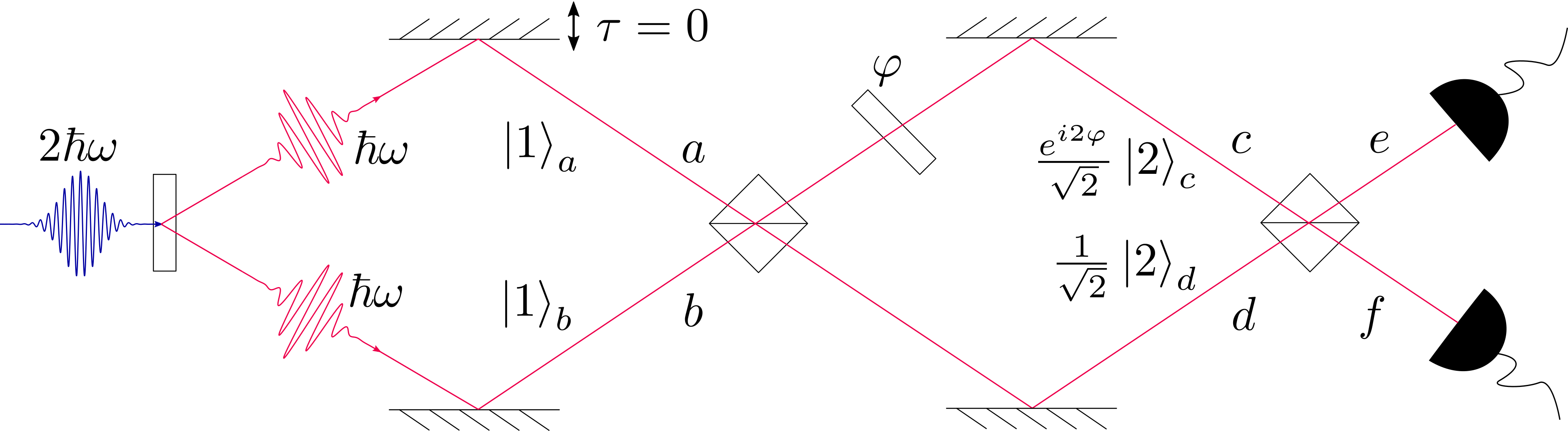
Fig. 16 A \(N=2\) NOON state interferometer.

Here we consider only the case for \(\tau = 0\), and have simplified our notation for the states to reflect that.

An important thing to observe here is that for path c, the two-photon state collects twice the amount of phase \(\varphi\) when going through the phase plate. This is a critical aspect that enables superresolution of the instrument for measurements of \(\varphi\). Furthermore, due to the entangled nature of the NOON state, there is also supersensitivity from reduced statistical fluctuations in the measurement of \(\varphi\). We will explore both of these aspects below.

First, lets consider the output state after the second interferometer. Similar to our analysis above, we find that

\[ \chat \rightarrow (\ehat + \fhat)/\sqrt{2} \]

and

\[ \dhat \rightarrow (\ehat - \fhat)/\sqrt{2} \]

Then we know that

\[\ket{\psi_\mathrm{in}} = \frac{ \big ( \cdagger \cdagger e^{i2\varphi} + \ddagger\ddagger \big ) \ket{0}}{2}\]

After substitution, we find that

\[\cdagger\cdagger \rightarrow \frac{1}{2}(\edagger + \fdagger)(\edagger + \fdagger) = \frac{1}{2}(\edagger\edagger + 2\edagger\fdagger + \fdagger\fdagger)\]

Likewise

\[\ddagger\ddagger \rightarrow \frac{1}{2}(\edagger - \fdagger)(\edagger - \fdagger) = \frac{1}{2}(\edagger\edagger - 2\edagger\fdagger + \fdagger\fdagger)\]

Meaning that

\[\ket{\psi_\mathrm{out}} = \frac{1}{4} \bigg \lbrace (\edagger\edagger + 2\edagger\fdagger + \fdagger\fdagger)e^{j2\varphi} + (\edagger\edagger - 2\edagger\fdagger + \fdagger\fdagger) \bigg\rbrace \ket{0}\]

Note

You may be wondering where the phase accumulation of \(2\varphi\) came from. We can represent a phase shift by evolution of the operator \(\ahat \rightarrow \bhat = \ahat e^{i\varphi}\) This means that \(\ahat = \bhat e^{-i\varphi}\). Thus, we have that \(\ket{2}_a = \frac{1}{\sqrt{2}}\adagger\adagger \ket{0} = \frac{1}{\sqrt{2}}e^{2i\varphi} \bdagger\bdagger \ket{0} = e^{2i\varphi} \ket{2}_b\).

Note that there are terms multiplied by \(e^{j2\varphi} \pm 1 = e^{j\varphi}(e^{j\varphi} \pm e^{-j\varphi})\). The reason this is important is because they can be expressed as multiples of \(\sin\) and \(\cos\) since \(e^{j\varphi} + e^{-j\varphi} = 2\cos{\varphi}\) and \(e^{j\varphi} - e^{-j\varphi} = 2j\sin{\varphi}\). Using this property and rearranging the terms in \(\ket{\psi}_\mathrm{out}\) above we find that

\[\ket{\psi_\mathrm{out}} = \frac{e^{j\varphi}}{2} \bigg \lbrace \cos({\varphi})(\edagger\edagger + \fdagger\fdagger) + j\sin({\varphi})\edagger\fdagger \bigg \rbrace \ket{0}\mathrm{.}\]

After applying all of the creation operators, we finally arrive at the output state

\[\ket{\psi_\mathrm{out}} = \frac{e^{i\varphi}}{\sqrt{2}}\cos({\varphi})(\ket{2}_e + \ket{2}_f) + ie^{i\varphi}\sin({\varphi})\ket{1}_e\ket{1}_f \mathrm{.}\]

Let’s take a moment to evaluate this. Similar to the output of our HOM experiment, we have various possibilities of coincidence detection or the separate detection of either a \(\ket{2}_e\) or \(\ket{2}_f\) state. However, there is now the added consideration that these outcomes depend on \(\varphi\). This is good as that is precisely what we want to detect. If we restrict ourselves to only looking at coincidence outputs in \(e\) and \(f\), we then find that they occur with probability

\[P_\mathrm{co}(\varphi) = \sin^2{\varphi}\]

meaning that we can adjust the probability of coincidence detection from 0 to 100% by simply adjusting \(\varphi\) from \(0\) to \(\pi/2\). It is convenient to get rid of the \(\sin^2\) term using a trigonetric identity

\[P_\mathrm{co}(\varphi) = \frac{1}{2} - \frac{1}{2}\cos(2\varphi)\mathrm{.}\]

It is at this point that you realize that the output oscillates as \(\cos(2\varphi)\). You can show that a classical interferometer oscillates as \(\cos(\varphi)\). This doubling of the oscillation rate for our NOON state interferometer is due to the reduced deBroglie wavelength of the higher order Fock state inputs! This faster variation with respect to \(\varphi\) provides superresolution compared to a classical interferometer. However, this isn’t the entire story. While superresolution is provided by the higher rate of oscillation with \(\varphi\), it is not guaranteed that the interferometer provides supersensitivity, meaning that it has reduced the smallest possible value of \(\varphi\) that can be measured. To demonstrate that supersensitivity is possible requires condiseration of the sensitivity of our measurements to small changes in \(\varphi\). To do this, we must consider the statistical variations of the photon number and how they impact our estimation of changes in \(\varphi\).

Demonstrating Supersensitivity

In most experimental situations we are trying to measure small changes in \(\varphi\). For convenience, let’s rewrite our phase as \(\varphi = \varphi_0 + \varphi_1\), where \(\varphi_1\) is a small change that we are trying to measure on top of an offset phase \(\varphi_0\). Let’s then imagine that we have some output signal \(C(\varphi)\). For a small enough \(\varphi_1\) we can use a Taylor expression to write

\[C(\varphi) \approx C(\varphi_0) + \frac{\mathrm{d} C}{\mathrm{d} \varphi}\bigg|_{\varphi_0} \varphi_1 \mathrm{,}\]

and from this we have that

\[\varphi_1 \approx \frac{C(\varphi) - C(\varphi_0)}{\frac{\mathrm{d} C}{\mathrm{d} \varphi}\big|_{\varphi_0}}\]

For the case of our noon-state interferometer, we might define \(C_k(\varphi)\) as the average number of coincidence counts after \(k\) incident photon events:

\[C_k(\varphi) = k P_\mathrm{co}(\varphi)\mathrm{.}\]

While we can use \(C_k(\varphi)\) to estimate small changes in phase \(\varphi_1\) as discussed above, the next interesting question regards the fundamental limit to the sensitivity of this measurement. To do that, we must account for the probabilistic nature of the coincident counting process. Given all technical noise could be removed, the last fundamental source of noise in our estimation of \(\varphi_1\) results from fluctuations in \(C_k\). Given that \(C_k\) exhibits a variance, the minimum variance in our estimate of \(\varphi_1\) from our measurements of \(C_k\) would then become

\[\delta \varphi^2 = \Delta C_k^2/(\mathrm{d}C_k/\mathrm{d}\varphi|_{\varphi_0})^2 \]

where \(\Delta C_k^2\) is the variance in the number of detected coincidence events after \(k\) trials. What is the variance of \(C_k\)? Given that each event has one of two outcomes (we either measure an event or we do not), the measurement is then analagous to that of a series of weighted coin tossess, and the variance follows the statistics of a binomial distribution.

For a binomial distribution we have that

\[\Delta C_k^2 = k P_\mathrm{co}(\varphi) (1 - P_\mathrm{co}(\varphi))\mathrm{.}\]

Let’s now consider our \(N=2\) NOON state interferometer specifically. We have that

\[\bigg | \frac{\mathrm{d}C_k}{\mathrm{d}\varphi} \bigg |^2 = k^2 \sin^2(2\varphi) \mathrm{.}\]

After feeding this into our expression for the variance of our phase estimation, we find that

\[\delta \varphi_{2002}^2 = \frac{1 - \cos^2(2\varphi)}{4k\sin^2(2\varphi_0)} = \frac{\sin^2(2\varphi_0 + 2\varphi_1)}{4k\sin^2(2\varphi_0)}\mathrm{.}\]

Given we are assuming sufficiently small \(\varphi_1\), we can do another Taylor expansion, finding that

\[\delta \varphi_{2002}^2 \approx \frac{1}{4k} + \frac{\cos(2\varphi_0)\varphi_1}{k\sin(2\varphi_0)}\mathrm{.}\]

The right hand coefficient on \(\varphi_1\) is important as it makes it clear that we want to operate where \(\cos(2\varphi_0) = 0\), which is where the probability \(P_\text{co} = 1/2\). This makes sense since this is where we have the maximum slope of \(C_k\) and thus the maximum sensitivity to changes in \(\varphi\). An example phase offset point where this happens is \(\varphi_0 = \pi/4\) for our \(N=2\) NOON-state interferometer, which results in

\[\delta \varphi^2_{2002} = \frac{1}{4 k} \mathrm{.}\]

We can rewrite this result with respect to the number of input photons, \(N_\mathrm{ph} = 2k\), which becomes

\[\delta \varphi^2_{N00N} = \frac{1}{2 N_\mathrm{ph}}\mathrm{.}\]

A classical interferometer follows the same statistical pattern (also equivalent to an N=1 NOON state at the input), but oscillates as \(\cos(\varphi)\) rather than \(\cos(2\varphi)\). If we were to go back through this same derivation, we would find that for a classical interferometer

\[\delta \varphi^2_\mathrm{classical} = \frac{1}{N_\mathrm{ph}} \mathrm{,}\]

with an optimal operating point of \(\varphi_0 = \pi/2\).

This means that our \(N=2\) NOON state interferometer has improved the fundamental variance of phase measurement by a factor of \(2\) compared to a classical interferometer, enabling superresolution.

In general, larger reductions in variance could be achieved if we could keep increasing the order of the input NOON state. One can show that the general result for an \(N\)-th order NOON state, the minimum variance scales as

\[\delta \varphi^2_\mathrm{NOON} = \frac{1}{N N_\mathrm{ph}} \mathrm{,}\]

with optimal operating points being \(\varphi_0 = \pi/(2N)\) (or any other \(\varphi_0\) where the probability of detection \(P = 1/2\)).

In the post-lab questions below, you will explore extensions to \(N = 3\) and \(N = 4\) NOON-state interferometers. In particular you will examine why realization of such interferometers is technically challenging to accomplish in the real world. However, we emphasize that these challenges aren’t fundamental – only technological. Yet another example of why we need quantum engineers.

Numerical Experiments

In this section we explore a numerical experiment that accounts for the photon detection statistics of a classical interferometer and NOON-state interferometry. The goal of this is to compare the noise performance of phase detection for each case.

For such numerical experiments we just need to understand the probability of detection. In general, the probability of detection goes as

\[P_\text{NOON} = \sin^2(\varphi N/2)\mathrm{.}\]

Note that if we set \(N=1\) this probability is that of a classical interferometer. Also, it is important to consider that at the input you require \(N\) photons. We need to consider this input photon number so that we make a fair comparison of the output statistics considering the same number of photons.

At the output, we have statistics that follow a binomial distribution. We either detect the desired event with probability \(P\), or we down with probability \(1-P\). Most scientific programming environments can simulate such binomial statistics. Using numpy we can call numpy.random.binomial(n, P) where n is the number of trials and P is the probability of detecting the desired outcome.

In the following, we simulate the cases for \(N=1\) \(N=2\), and \(N=4\) considering a fixed input of \(N_\mathrm{ph}\) photons. To see the sensitivity to \(\varphi\) we consider that it is modulating in time such that

\[\varphi = \varphi_0 + \delta\varphi \sin (2\pi f t)\mathrm{.}\]

This is rather arbitrary for visualization, and we look over a period of 1 second with \(f=4\) Hz. We consider \(\delta\varphi = 0.05\). The value of \(\varphi_0\) is chosen for each case to put the probability at the highest slope where \(P=0.5\).

import numpy as np
import matplotlib.pyplot as plt
import ipywidgets


fig = plt.figure();
fig.set_size_inches(15, 7);

del_phi_0 = 0.05
N_ph = 1000

t = np.linspace(0, 1, 1000)
f = 4
omega = 2*np.pi*f
del_phi = del_phi_0*np.sin(omega*t)

phi_cl = np.pi/2
phi_2002 = np.pi/4
phi_4004 = np.pi/8

P_cl = np.sin((phi_cl + del_phi)/2)**2
P_2002 = np.sin(phi_2002 + del_phi)**2
P_4004 = np.sin(2*(phi_4004 + del_phi))**2

N_cl = np.random.binomial(N_ph, P_cl)
N_2002 = np.random.binomial(N_ph/2, P_2002)
N_4004 = np.random.binomial(N_ph/4, P_4004)

ax1 = fig.add_subplot(1, 3, 1)
ax2 = fig.add_subplot(1, 3, 2)
ax3 = fig.add_subplot(1, 3, 3)

ax1.clear()
ax1.plot(t, N_cl, 'o');
ax1.set_ylabel('Counts', fontsize=15)
ax1.set_title('1001 (Classical)', fontsize=15)

ax2.clear()
ax2.plot(t, N_2002, 'o');
ax2.set_xlabel('Time (s)', fontsize=15)
ax2.set_title('2002', fontsize=15)

ax3.clear()
ax3.plot(t, N_4004, 'o');
ax3.set_title('4004', fontsize=15);

Show code cell output Hide code cell output

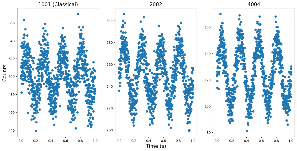
Fig. 17 Comparison of classical and NOON state interferomters. The plot shows the recorded number of counts (photon counts for the classical case, or multiphoton events in the NOON state cases) for a fixed number of 1000 photons input to each interferomter. The phase is modulated sinusoidally in time with an amplitude of 0.05 radians and frequency of 4 Hz. Note the improved noise performance of the NOON-state interferometers. If you reduce the phase modulation amplitude, you will notice that the NOON state interferometers can resolve phase modulations of lower amplitude than the classical interferometer.

Note how the modulation is clearly better resolved defined with higher signal-to-noise ratio as the photon order increases. This is even in-spite of progressively fewer collected events!

You are encouraged to launch this notebook where you will find an interactive version of this code below. Play with the number of input photons and the phase modulation amplitude and observe how the statistics change. Note that if you progressively decrease the amplitude of the phase modulation, you will find a value where the modulation is almost impossible to discern for the classical \(N=1\) case, but easily discernable for the \(N=4\) case.

Post-Lab Questions

1. In practice, we find that imperfections in allignment photon detection prevent the achievement of improved sensitivity beyond what is possible with a classical interferometer. To account for such imperfections, we can write the propability of coincidences more generally as \(P(\varphi) = \eta \big ( 1 - V \cos(N\varphi) \big )/2\) for an \(N\) photon number NOON state. Express the variance of the estimated phase for general \(\eta\) and \(V\).

2. Given \(\eta = 1\), what are the constraints on \(V\) needed to ensure phase sensitivity beyond that of a classical interferometer?

3. Derive the output state for \(N = 3\) and \(N = 4\) NOON state interference (i.e. output states \(e\) and \(f\) given you have \(N = 3\) and \(N = 4\) NOON state inputs to the \(c\) and \(d\) ports in Fig. 16). For performing phase-measurmeents with high visibility for \(N = 3\) and \(N = 4\), what are the requirements on post-selection? Is a simple coincidence detector still sufficient?

4. Discuss the engineering challenges involved with regard to state generation and post selection needed for true quantum-enhanced phase measurements with this approach. (For this question, it may be helpful to consider the challenges faced in the experiments discussed in Refs. [NOOBrien+07, OHN+08].

References

Bra17

Agata M. Brańczyk. Hong-Ou-Mandel Interference. October 2017. arXiv:1711.00080 [quant-ph]. URL: http://arxiv.org/abs/1711.00080 (visited on 2022-07-04), doi:10.48550/arXiv.1711.00080.

HOM87

C. K. Hong, Z. Y. Ou, and L. Mandel. Measurement of subpicosecond time intervals between two photons by interference. Physical Review Letters, 59(18):2044–2046, November 1987. Publisher: American Physical Society. URL: https://link.aps.org/doi/10.1103/PhysRevLett.59.2044 (visited on 2022-07-13), doi:10.1103/PhysRevLett.59.2044.

NOOBrien+07(1,2)

Tomohisa Nagata, Ryo Okamoto, Jeremy L. O'Brien, Keiji Sasaki, and Shigeki Takeuchi. Beating the Standard Quantum Limit with Four-Entangled Photons. Science, 316(5825):726–729, May 2007. Publisher: American Association for the Advancement of Science Section: Report. URL: https://science.sciencemag.org/content/316/5825/726 (visited on 2020-11-12), doi:10.1126/science.1138007.

OHN+08(1,2)

Ryo Okamoto, Holger F. Hofmann, Tomohisa Nagata, Jeremy L. O'Brien, Keiji Sasaki, and Shigeki Takeuchi. Beating the standard quantum limit: phase super-sensitivity of\$\less\$i\$\greater\$N\$\less\$/i\$\greater\$-photon interferometers. New Journal of Physics, 10(7):073033, July 2008. Publisher: IOP Publishing. URL: https://doi.org/10.1088/1367-2630/10/7/073033 (visited on 2022-08-05), doi:10.1088/1367-2630/10/7/073033.