LAB - Quantum Sensing with Solid State Spins (Week 1)

In this lab, you will explore using RF electronics to probe the microwave cavities and coupling the cavities to NV centers in diamond to enable quantum magnetometry.

Specific aims are:

1. Understand the optical setup
2. Characterize the microwave cavities and the Helmholtz coil
3. Simulate strong coupling between NV centers and the microwave resonator
4. Achieve strong coupling between NV centers and the microwave resonator
5. Improving the avoided-crossing contrast

Please note the questions throughout the lab instructions. You will be expected to address these in your lab writeup. You are also expected to keep lab notebooks (can be digital, paper, or both) for notes, data, and analysis.

Day 1: Understand the optical setup

Pre-Lab Questions

In the first session of this experiment, you will first be characterizing the microwave cavity by measuring its resonance frequency and quality factor. Recall that a cavity \(Q\) is defined to be the ratio of its resonance frequency to its decay rate (also known as the cavity linewidth).

1. Calculate the \(Q\) of a cavity with resonance frequency at 3 GHz and linewidth of 100 kHz.

2. Typically the cavity linewidth is defined at the full width at half maximum. Insert a cell below and write a Python script plotting a resonance peak centered at 3 GHz with linewidth of 100 kHz. Make the x-axis frequency with a span of 1 MHz and the y-axis normalized cavity transmission. Note that the cavity lineshape is usually Lorentzian.

The second part involves characterizing the Helmholtz coil by measuring its generated magnetic field. Recall that due to the Zeeman effect, magnetic field is used to shift the energy (frequency) difference between the \(m_s=0\) and \(m_s= \pm 1\) states of NV centers. Importantly, the correct amount of magnetic field must be applied to ensure one of the energy differences matches the microwave cavity’s resonance frequency.

3. The amount of frequency shift due to magnetic field strength \(B\) is \(\delta f = \mu B\), where \(\mu = \mu_B g/h\). \(\mu_B\) is the Bohr magneton, \(g\approx 2\) is the Lande factor, and \(h\) is the Planck constant. Calculate \(\mu\) in units of MHz/Gauss. Note the SI unit for magnetic field is Tesla, where 1 Tesla = \(10^4\) Gauss.

4. Assume you have a cavity resonant at 3GHz. Which energy difference would you align to the cavity resonance: \(m_s=0\) and \(m_s=+1\), or \(m_s=0\) and \(m_s=-1\)? Why? Recall the starting point (due to crystal field splitting) of the energy difference between \(m_s=0\) and \(m_s=\pm 1\) is 2.87 GHz.

5. Calculate the needed magnetic field strength (in Gauss) if the cavity resonance frequency is at 3 GHz.

Optical Setup

In this lab, you will be using a home-built optical setup containing the following main components:

• a 3W 532nm free space laser (this is a class-4 laser requiring laser safety!)

• a magnetic shield

• a microwave cylindrical resonator

• a loop coupler

• a Helmholtz coil

• diamond samples (~3mm x 3mm x 0.5mm) containing NV centers

• cavity mounts (PTFE disks)

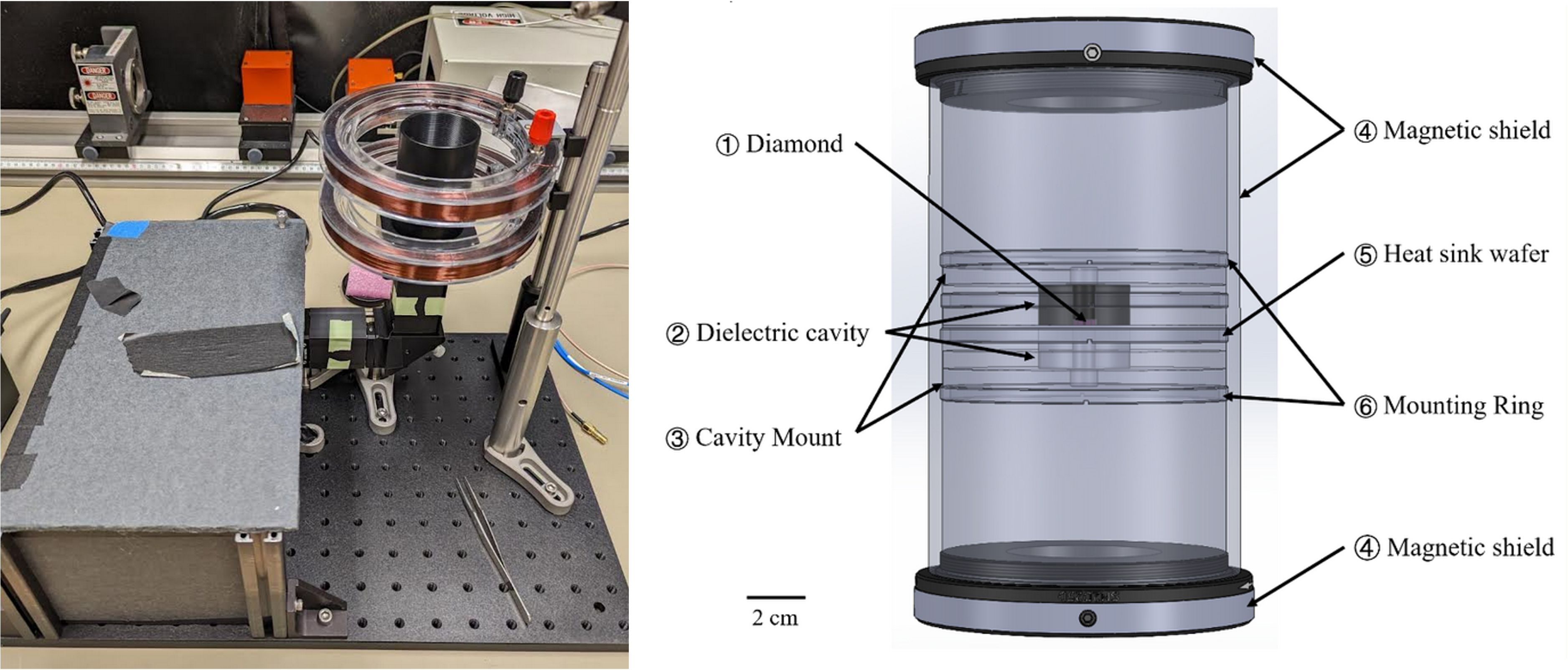
Fig. 55 (left) Picture of the experimental setup. (right) Diagram depicting the magnetic resonator and diamond placed inside a magnetic shield.

Not shown in the picture of the setup are the electronics and the RF components needed to probe the microwave cavity. You will be tasked to put together the RF circuitry for running the experiment.

As mentioned during the demo session, the experiment is based mainly on E. Eisenach et al, Cavity-enhanced microwave readout of a solid-state spin sensor, which you may find to be a valuable reference.

Other helpful references may be:

• JF Barry et. al. Sensitivity optimization for NV-diamond magnetometry

• D. Fahey et. al., Steady-state microwave mode cooling with a diamond NV ensemble

• ME Trusheim et. al. A Polariton-Stabilized Spin Clock

Aim 1: Characterize the microwave cavities and the Helmholtz coil

Lab Exercise

For the following steps, please take extra care when handling the microwave cavities and the loop coupler!

i) Estimate the cavity’s resonance frequency

Internally, the optical setup’s microwave cavity really consists of two stacked resonators. We provide an additional one of these resonators for you to examine. Take it and measure its outer radius and length. Use the measured geometry parameters and estimate the cavity’s resonance frequency.

Can you measure the resonator’s resonance frequency via the VNA, whose bandwidth covers 100 kHz to 6 GHz?

What would be the expected resonance frequency if you stack two of these resonators on top of another, with their central holes as aligned as possible?

Can you measure the resonator’s resonance frequency via the VNA?

ii) Build the RF circuitry for probing the cavity’s resonance frequency

The VNA has a send port (Port 1) and a receive port (Port 2). Port 1 sends out a microwave tone by an internal signal generator, and port 2 measures the transmitted/reflected signal to compute the S-parameters. Use the provided circulator and note the numbers written on its, connect its ports to the VNA and the loop coupler appropriately such that the loop coupler can be used to probe the cavity’s signal. Check with the TA after you are done.

iii) Measure the microwave resonator’s frequency

Now with the loop coupler properly connected to the VNA via the circulator, open the iris at the top of the magnetic shield, enough for the loop to fit through. Mount the loop coupler such that it is directly above the resonator in the cage-mounted displacement stage. The stage can be secured by tightening one of the screws on its corner.

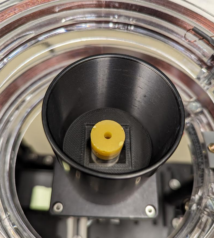
Fig. 56 Microwave resonator inside the magnetic shield.

Open the libreVNA GUI and connect to the device. Make sure you are monitoring the “S21” window. Change the center frequency to what you estimated above for the resonator. Change the span to 20 MHz. By adjusting the position of the loop coupler relative to the resonator, you should be able to observe the cavity resonance dip. Based on your measurements, take note of whether what you expect to probe; \(m_s = +1\) or \(m_s = -1\).

Once you have done so, play around with the position of the loop coupler and observe how the cavity’s observed loaded \(Q\) and resonance frequency \(\omega_c\) change. Write down your observations and explanations to these changes as a function of position. In Aim 2, you will need to methodically measure the cavity resonance frequency and quality factor as a function of \(z\).

iv) Characterize the coil

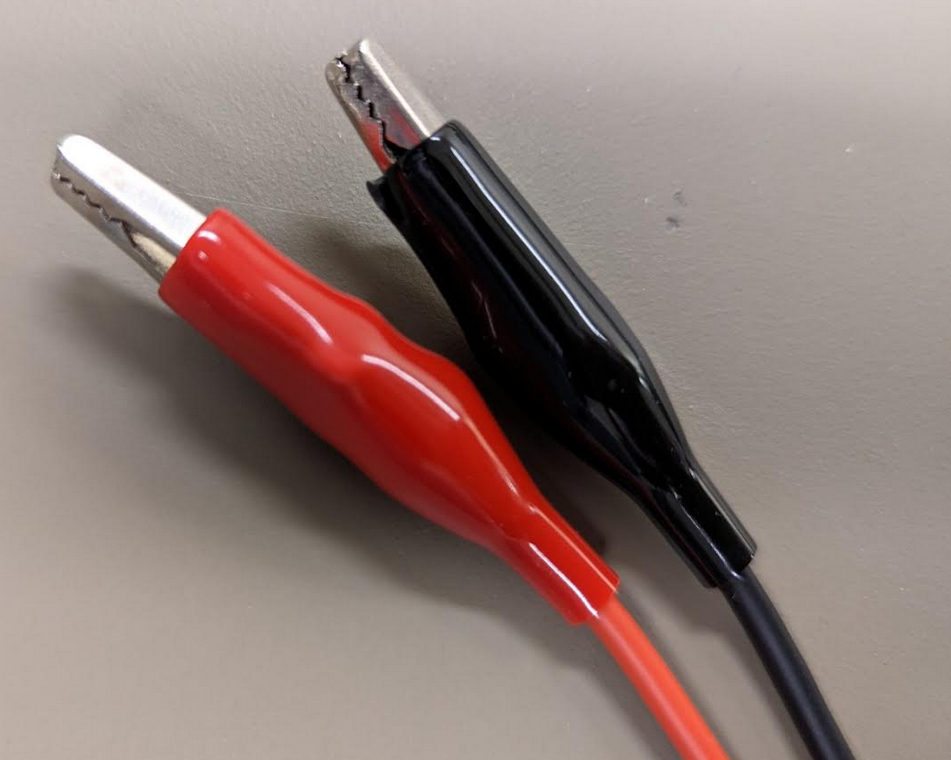
Fig. 57 Alligator clips.

We will use a solenoid coil to generate the DC magnetic field that tunes the NV spin magnetic frequency. Connect the red and black alligator clips to the leads in both coils. Note that red typically indicates the positive end, and black indicates the negative end. Check with the TA if you are unsure.

After you are done, grab the alligator clips’ BNC cable ends and connect them to a BNC-Tee connector. Then, attach the BNC-banana connector adapter to the BNC-Tee connector, and insert the adapter into Channel 1 of the R&S power supply (HMP4040).

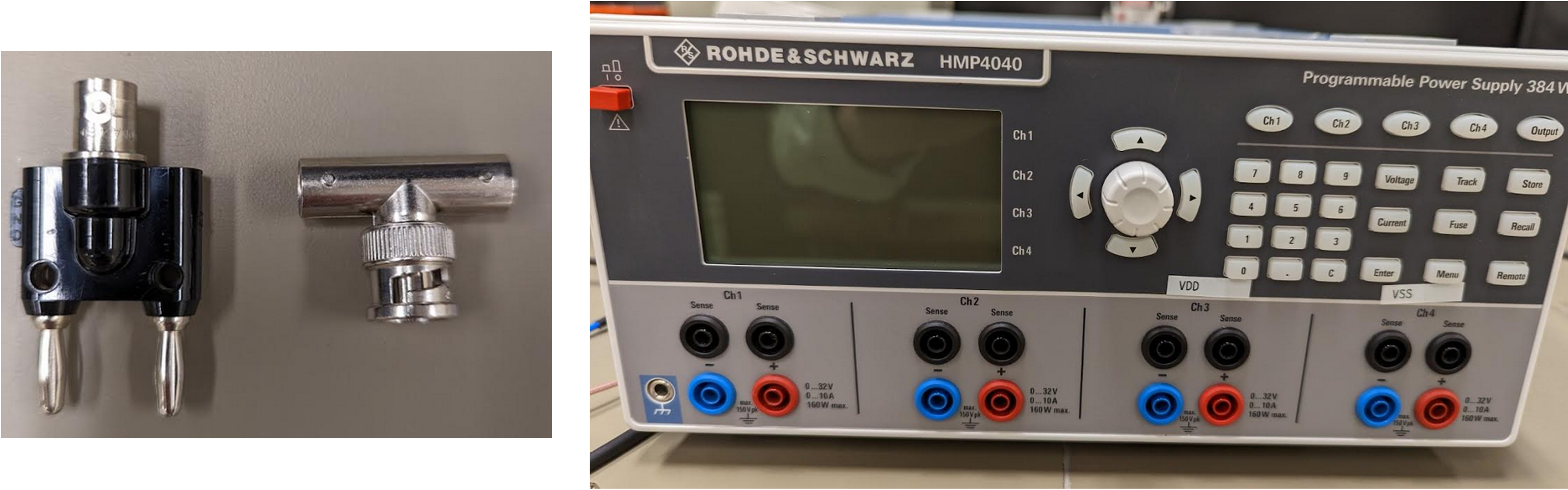
Fig. 58 (left) An adapter for banana plugs and BNC, BNC Tee connector. (right) Rhode & Schwarz power supply, HMP4040.

Next, turn on the Gauss meter.

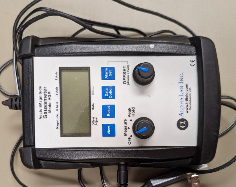
Fig. 59 Gauss meter.

What is the intrinsic reading displayed on the Gauss meter? Why is it non-zero?

Set Channel 1’s voltage to 1 V, and click on “Output” on the top right of the front panel of the power supply. Put the Gauss meter’s probe in between the loops and note down the measured magnetic field.

Estimate the number of loops per coil. You may find this solenoid calculator useful.

Increase the voltage in increments of 1 V all the way to 20 V, and write down the measured magnetic field for each voltage setting. Please do not set the voltage beyond 20 V without consulting the TA

Generate below a plot of magnetic field in Gauss (y-axis) vs Channel 1’s voltage (x-axis).

Aim 2 (Day 2): Simulate strong coupling between NV centers and the microwave resonator

Prelab

Here are some questions to better prepare you for the lab exercise.

1. Consult this product link for one of the diamond types. Obtain the nitrogen concentration under “Materials Properties” and assume that all nitrogen defects in the crystal lattice are converted to NV centers. Estimate the density of NV centers in diamond in units of NV/m\(^3\).

   Hint: you may need to look up the atomic density of diamond and convert to its units to number of atoms/m\(^3\).

2. Given our diamond dimensions, 3mm x 3mm x 0.5mm, what is the effective coupling strength \(g\)? Assume a single spin coupling strength is \(g_0=0.01\) Hz. You may find the paper by Eisenach et al. helpful.

Now you should be equiped to do the lab exercise!

Lab Exercise

In this lab session, you will be strictly working on creating a Python script that simulates the strong coupling dynamics between NV centers and the microwave resonator. In scientific research, it is often extremely valuable to be able to predict how the experimental results may vary depending numerous parameters. By producing a digital twin, you will be able to better understand the feasibility of using such a solid state spin-based system for performing quantum sensing.

i) Estimate the microwave cavity’s intrinsic quality factor

Last time, you observed changes in the cavity resonance as you adjusted the loop coupler. This session, you will measure quantitatevely to determine the cavity’s intrinsic Q. Remember that the loaded \(Q\propto 1/\kappa_c\) and the coupling rate to the loop coupler \(\kappa_1\) are both functions of \(z\).

Measure and record the loaded \(Q\) at various loop coupler heights. Be sure to have the loop coupler as directly above the microwave resonator to remove any \(x,y\) dependence. The cable to the loop coupler can bend slightly. You will have some flexibility in how to measure height. Rough measurement is ok. Note that you do not need to directly measure \(z\) (height between the loop and top of the cavity); a height meausrement relative to a convenient feature will work. If you record multiple heights with a common offset, you will be able to fit for this offset and recover that actual \(z\). Fit your plot with an exponential function, e.g. \(\propto 1-exp(-z)\) (add an appropriate offset term if necessary). Use your fit to estimate the intrinsic quality factor, \(Q_0\propto 1/\kappa_0\).

Then, generate a plot of \(\kappa_1\) as a function of \(z\).

ii) Plot the frequency difference between \(m_s=0\) and \(m_s=\pm 1\) states as a function of magnetic field (in Gauss)

iii) Generate a 1D plot of the cavity reflection coefficient

Recall that the cavity reflection coefficient is defined as:

\[\Gamma(\omega) = -1+\frac{\kappa_{c1}}{\frac{\kappa_c}{2}+j(\omega-\omega_c)+\frac{g^2}{\frac{\kappa_s}{2}+j(\omega-\omega_s)+\alpha}}\]

For simplicity, let’s first take \(g=0\). Generate a 1D plot of the real part of \(\Gamma(\omega)\) as a function of \(\omega\). Choose and define \(\omega_c,\kappa_c,\kappa_{c1}\) based on what you measured in Aim 1 and calculated above.

iv) Generate 2D plots of the cavity reflection coefficient

Now, use the effective coupling strength \(g\) you computed in the Prelab, generate 2D plots of the following, with the \(x\)-axis being magnetic field strength and \(y\)-axis being frequency:

• In-phase component of \(\Gamma(\omega)\)

• Quadrature component of \(\Gamma(\omega)\)

• Amplitude of \(\Gamma(\omega)\)

• Phase of \(\Gamma(\omega)\)

Initially, choose \(\omega_c,\kappa_c,\kappa_{c1}\) based on what you meausred. If needed, adjust these values appropriately to ensure you can observe avoided crossing similar to what was observed by Eisenach et al. (Figure 2). You may assume \(\alpha=0\). \(\kappa_s=2/T_2\) where \(T_2\) is the coherence time of the NV centers. You may assume \(T_2=20~\mu\)s.

You may find using the Python module ipywidgets helpful. By creating a widget with scroll bars, you may be able to freely change the parameters without manually typing in different values. Specifically, the interact_manual method (see documentation here).