LAB – Quantum Sensing With Solid State Spins (Week 2)

LAB – Quantum Sensing With Solid State Spins (Week 2)#

Aim 4 and 5: Achieve strong coupling between NV centers and the microwave resonator; Improve the avoided-crossing contrast#

This portion of the lab is not explicity split into days. A general guideline would be to aim to complete the data collection code on the first day, and to collect data and optimize coupling on the second day.

If you have time, you should try to collect data on the first day, which would be valuable to achieve stronger contrast on the second day.

Pre-lab#

Please complete the pre-lab 3 from the text prior to this lab session.

Setting up Code for Data Collection#

i) Collecting data from the VNA#

You will be extacting data from the VNA using Python. This is covered in TRAINING - Interfacing with the Vector Network Analyzer. Try extracting a plotting a trace from the VNA.

ii) Interface with the power supply#

Similar to interfacing with the VNA during T3E3-TRAINING, you will also need to be able to control the power supply via Python. First, install the packages qcodes, qcodes_contrib_drivers, and pyserial. Then, ensure the power supply’s USB port is connected to the computer. Run the following cell to determine which serial port it occupies.

import serial.tools.list_ports
ports = serial.tools.list_ports.comports()

for port, desc, hwid in sorted(ports):
        print("{}: {} [{}]".format(port, desc, hwid))

Alternatively, you can also run python -m serial.tools.list_ports directly in terminal.

Following the example shown here, make sure you can set Channel 1’s voltage and turn Channel 1’s output on/off via Python commands.

NOTE: The power supply uses VISA to communicate with the computer. The VISA resource name corresponds to the COM port(e.g. COM2 -> ASRL2)

### Your code goes here

iii) Write an experimental sequence to produce a 2D map of frequency vs magnetic field#

From T3E3-TRAINING, you were able to interface with the VNA via Python. And from part (i), you were able to interface with the power supply, which effectively drives the Helmholtz coil and thereby the amount of the mangetic field being generated.

Below, please write an experiment sequence that performs a 2D sweep over both frequency and magnetic field. The sweep over frequency is essentially done for you by the VNA. Your task here will be to grab a trace off the VNA (with carefully defined frequency center and span corresponding to the cavity signal), and sweep over a range of voltages. The voltage range, i.e. the sweeping range of the magnetic field strength, should cover the required field strength to shift the NV centers’ resonance to match the cavity resonance. This was calculated by you in Aim 1’s Prelab.

Importantly, for each magnetic field strength, you should obtain an average over multiple frequency traces. In your script, please also compute the variance of each point. You may need VNA functionality not directly covered in the training. The LibreVNA SCPI Programming Guide may be useful.

You should run a pseudo-experiment without the laser on to make sure the experimental sequence runs smoothly. Please also check that you can generate a 2D map of your acquired “data”.

Running the Coupling Experiment#

i) Aligning the laser to excite the diamond#

As you saw in previous labs, the resonator is composed of two parts with a hole in the center, and a silicon carbide wafer in between the two parts.

The diamond should be just the right size to lie flat on the silicon carbide wafer at the bottom of the top half of the resonator hole. The diagram shown below is a reference to what the full stack looks like:

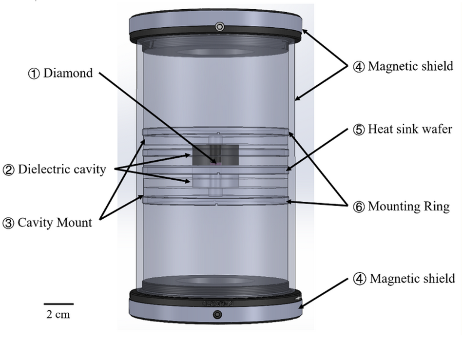
../_images/week2_stack.png — Fig. 61 Diagram depicting a combined stack of the magnetic resonators and a diamond sample placed inside a magnetic shield.#

At this point, call your TA over to the station to turn on the laser (heavily attenuated such that the optical power is much less than 3 W). Please wear proper laser safety glasses now.

Your TA will then align the laser light to ensure it is incident on the diamond by turning the knobs of the 45-degree mirror at the bottom of the cage (see picture below).

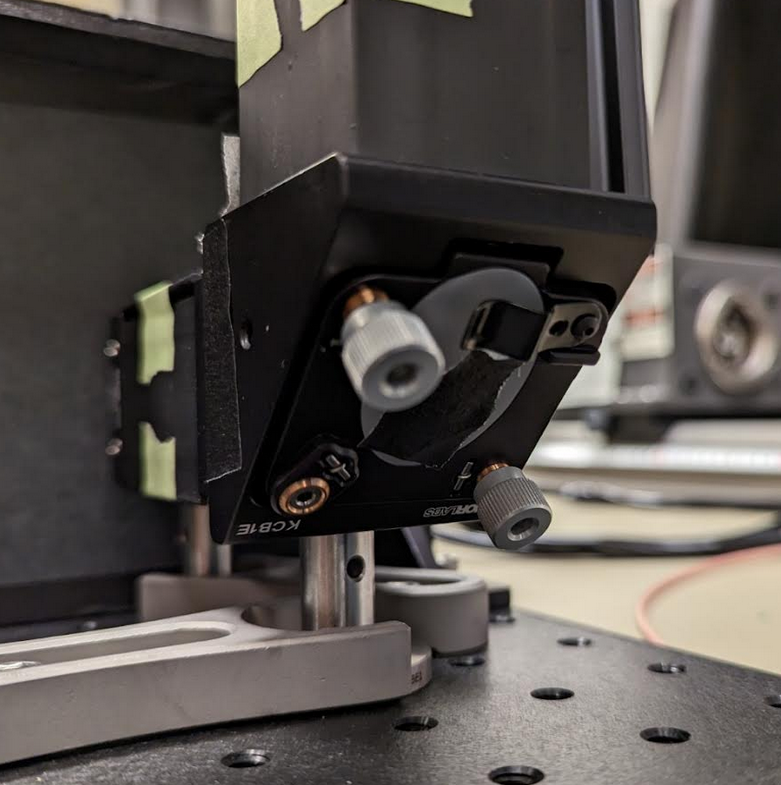
../_images/week2_mirror_knobs.png — Fig. 62 The 45-degree kinematic mirror mount with two knobs used for aligning the laser beam with respect to the diamond samples.#

With the laser at minimum power, still with your laser safety glasses on, you should be able to see fluorescence emanating from the diamond. The fluorescence stems from the atomic transitions between the ground and excited states of the triplet manifold \(^3 E \leftrightarrow ^3 A\) in NV centers’ level structure. Recall from T3E3-TEXT that the direct emission from the exited state to the ground state corresponds to 637\(~\)nm. If we placed a 638\(~\)nm optical longpass filter in front of the diamond, would you still be able to observe fluorescence? Why or why not? You may find the photoluminescence spectrum below helpful.

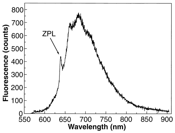
../_images/week2_nv_spectrum.png — Fig. 63 NV center’s photoluminescence spectrum. Figure adapted froom Gruber *et al.*.#

ii) Optimize the position of the loop coupler#

In order to see avoided-crossing, you want to maximize the effective cooperativity of the spin-cavity system. The cooperativity \(C\) scales with \(1/\kappa_c\). In other words, we must ensure the quality factor is as high as possible, while keeping the loop coupler sufficiently close to be able to probe to cavity’s frequency response. Do your best to optimize the position of the loop coupler by changing its height using the micrometer on the displacement mount to achieve the highest quality factor, i.e. smallest cavity linewidth. Unfortunately, its \(x,y\) positions will be fixed by the iris, which is intended as both an additional magnetic shield and laser block. We can still somewhat tweak this by by slightly bending the coaxial cable feeding the loop.

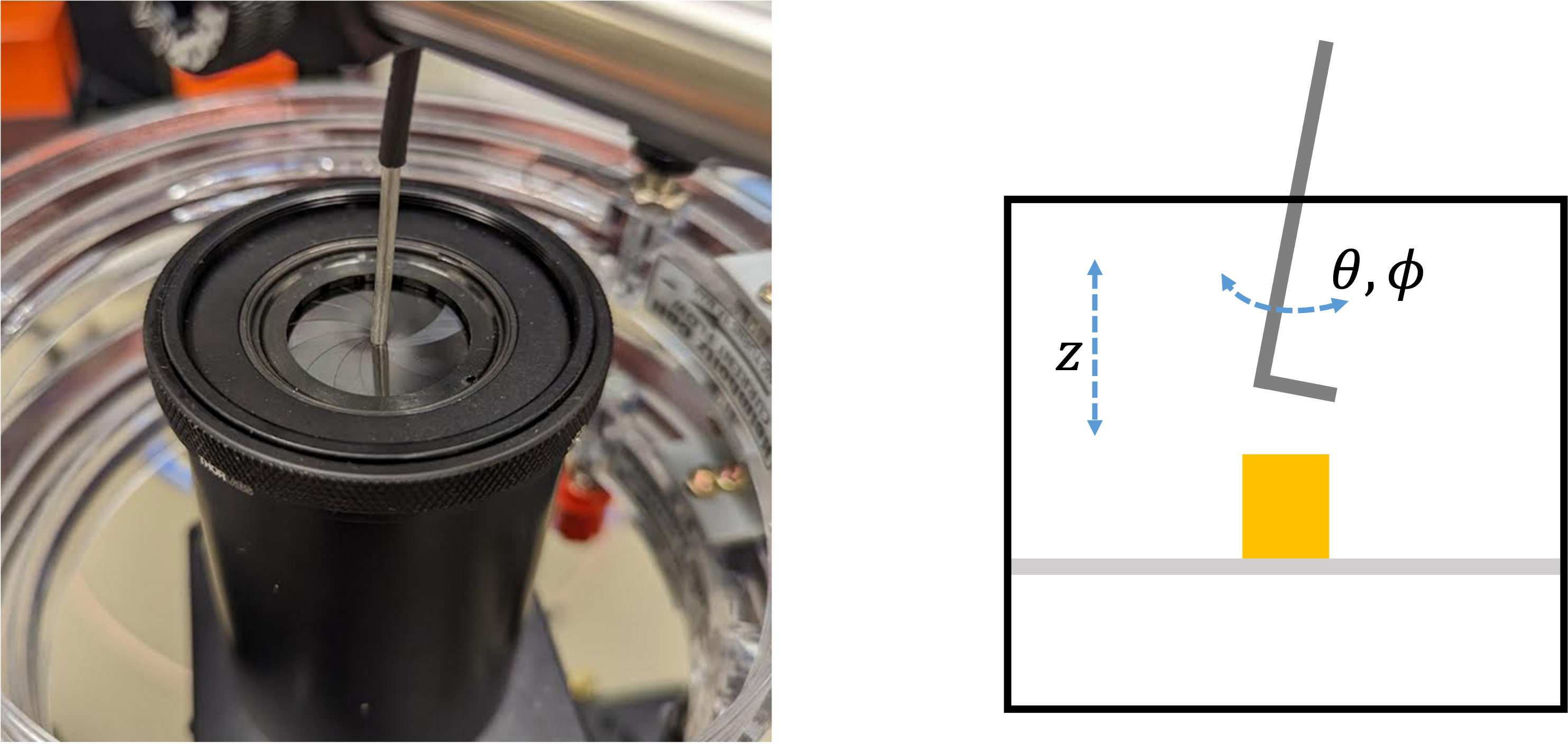
../_images/week2_iris_adjust.png — Fig. 64 (left) Picture of an iris wrapping around the looper coupler. (right) Diagram showing the degrees of freedom for optimizing the loop coupler’s position.#

The system is still quite sensitive, so avoid knocking it once you have achieved a good alignment. It may require further tweaking after the laser has been on for some time due to thermal heating.

### Your code goes here

iii) Run the experimental sequence and determine if you have achieved strong coupling#

Now, it is time to reproduce the avoided-crossing data you have seen in the demo and in your simulation results from Aim 2!

Call your TA over when you have reached this step. Remeber to put on your laser safety glasses. After your TA closes the iris (if you have not done so already) and places the safety shielding (an additional laser block) above it, the laser will be turned on to its max power. At this point, run the experimental sequence you have scripted.

If the cavity quality factor is narrow enough, and the coupling strength between NV centers and the microwave resonator is sufficiently strong, the spin-cavity system should achieve strong coupling. In this case, your 2D map should contain “kinks” at each of the three hyperfine transitions.

If you are having troubles, discuss with your teammates about ways to increase the coupling strength, SNR, …etc. Consult with your TA afterwards.

Once you have obtained data exhibiting strong coupling, try increasing the number of VNA traces being averaged over per each magnetic field strength to see if the contrast improves further.

iv) Estimate the sensitivity#

With your acquired data, please estimate the maximal magnetic field sensitivity you have achieved. The phase noise of the spectrum analyzer in the VNA is measured to be -103\(~\)dBc/Hz at 1\(~\)GHz (for simplicity, we will assume the noise level is the same for our frequencies).

You should:

First, convert the phase noise \(d\phi\) to \(V_{\text{rms}}/\sqrt{\text{Hz}}\). For this, you will need to obtain the input power from either the libreVNA GUI or use the Python interface.
Second, re-plot the 2D data for \(dV/dB\), where \(B\) is the magnetic field strength and \(V\) is the r.m.s. voltage \(V_{\text{rms}}\). Note that the data you extract from the VNA via Python is in dBm (power).
Third, find the maximum \(dV/dB\) and compute \(d\phi/(dV/dB)_{\text{max}}\) in pT/\(\sqrt{\text{Hz}}\). This would be your maximum magnetic field sensitivity, assuming your noise floor is limited mainly by the VNA’s phase noise.